7.2.3 Processing steps
Author(s): Leanne Guy, Berry Holl, Marc Audard, Alessandro Lanzafame, Isabelle Lecoeur-Taïbi, Nami Mowlavi, Lorenzo Rimoldini, Joris De Ridder, Luis Sarro, Sara Regibo, Grégory Jevardat de Fombelle
Overview
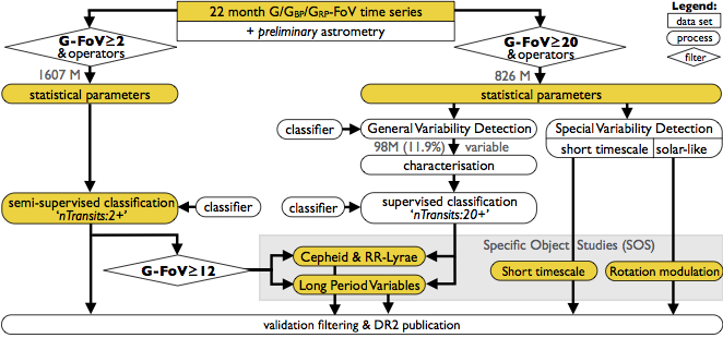
An overview of the variability processing is presented in Figure 7.1. There are two main paths: one starting from -FoV transits (left) and one from -FoV transits (right). The former results in the published nTransits:2+ classification results, and the latter results in the published Specific Object Tables of: vari_short_timescale (Section 14.3.8) and vari_rotation_modulation (Section 14.3.6). The published Specific Object Tables of: vari_rrlyrae (Section 14.3.7), vari_cepheid (Section 14.3.1), and vari_long_period_variable (Section 14.3.5) result from a mixed feed of classification candidates from the published nTransits:2+ classifier (for sources with a minimum of 12 -FoV transits) and from the unpublished nTransits:20+ classifier. The data was published from the highlighted yellow boxes for sources that passed the validation filtering.
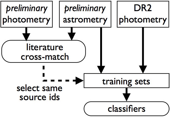
Figure 7.2 details how the sources were cross-matched on a preliminary version of the photometry.
Initial light curve pre-processing
Definition of observation time
Observation times are expressed in units of Barycentric JD (in TCB) days, computed as follows:
-
1.
The observation time is converted from On-board Mission Time (OBMT) into Julian date in TCB (Temps Coordonnée Barycentrique).
-
2.
A correction is applied for the light-travel time to the Solar system barycentre, resulting in Barycentric Julian Date (BJD).
-
3.
Although the centroiding time accuracy of the individual CCD observations is (much) below 1 ms, the per-field-of-view observation times processed and published in Gaia DR2 are averaged over typically 9 CCD observations over a time range of about 44 sec.
Conversion from flux to magnitude
In the variability pipeline, magnitudes rather than fluxes are used in the various processing modules. To convert to magnitude, the zero-point magnitudes for , , provided by CU5 in the Vega system are used (Section 5.3.6).
Observation filtering
The variability processing includes several operators that are applied to the ingested and reconstructed photometry. Typical time series operators perform flux to magnitude conversion, outlier removal and error cleaning on the input time series to create derived (transformed and/or filtered) time series suitable for processing by specific algorithms. Chaining of these time series operators creates a hierarchy of derived time series that is used as required by the scientific analyses while ensuring that provenance is preserved.
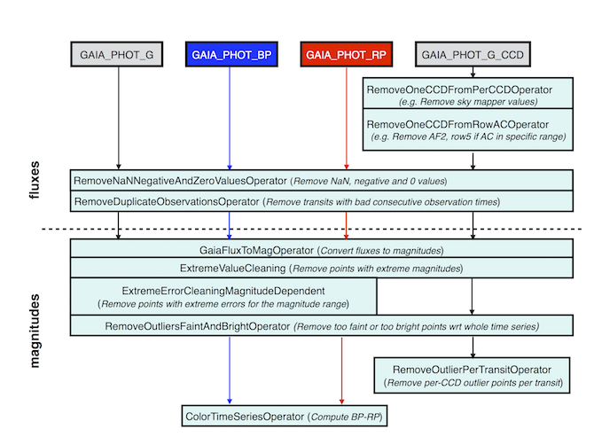
The following list of operators are applied in sequence to the input photometric time series, a schematic showing the hierarchy of these operators is presented in Figure 7.3:
-
1.
RemoveNaNNegativeAndZeroValuesOperator: it removes photometric transits that contain NaN, negative, or 0 flux values.
-
2.
RemoveDuplicateObservationsOperator: it removes pairs of transits (within each Gaia band) that are too close in time (within 105 min) to be observations of the same source. Such transits can occur in bright sources for which multiple artefact detections are assigned (these are known as ‘far double detections’). Since CU7 did not have access to the flags identifying the double detections transits, this ad-hoc method was applied by which close-in-time pairs of transits were removed.
-
3.
RemoveOneCCDFromRowAcOperator: it is designed to remove one CCD point (defined by its CCD number, between 0 and 9, 0 standing for the Sky Mapper and 1 to 9 for the Astrometric Field CCDs) from each transit of per-CCD data whose measurements correspond to a certain CCD row and whose across-scan (AC) coordinate is outside a certain range (minimum AC=3, maximum AC=1990). It was motivated by the fact that the photometric calibration team reported problematic flux measurements for the second Astrometric Field (AF) CCD of row 5 when AC is greater than 1200. Hence, in Gaia DR2 this operator was tailored to remove the AF2 points for transits with CCD row=5 and AC coordinate .
-
4.
GaiaFluxToMagOperator: it converts fluxes to magnitudes by using the zero-point magnitudes delivered by CU5.
-
5.
ExtremeValueCleaning: it removes points above a specific magnitude limit. Cuts were applied at , , and mag.
-
6.
ExtremeErrorCleaningMagnitudeDependent: it removes individual transits above or below magnitude-dependent values. The values were determined as follows: from a sample of the CU5 photometric catalogue and for each band (limited to 6000 sources per 0.1 magnitude bin), we studied the quantile distribution of the transit magnitude errors. A decision was made to use the 99.7% quantile for the upper value, and the 0.01% for the lower value for data. For and , a cut was applied only above the upper value of the 99.9% quantile. Figure 7.4 shows the distributions of the transit magnitude errors as a function of the transit magnitudes, for the 3 Gaia bands, together with the thresholds used for this operator. The latter was not applied to per-CCD data.
-
7.
RemoveOutliersFaintAndBrightOperator: it removes data points as follows (with configuration parameters described, where relevant, in the respective data product sections).
-
(a)
A point with a too large error (intrinsically or compared to some number of times the interquartile range of the uncertainties) is an outlier. It is removed before the next step.
-
(b)
Measurements at the extremes of the magnitude distribution of a time series are identified from their deviations from the median magnitude when these exceed a certain number of times the interquartile range (with different thresholds possible at the bright and faint ends). A point with an ‘extreme’ magnitude (on the faintest or brightest side, compared to the median magnitude) is an outlier unless it has similar outlying neighbours in time or projected in magnitude.
-
(a)
-
8.
RemoveOutlierPerTransitOperator: it removes per-CCD outlier data points per transit. This operator only applies to per-CCD data.
-
9.
ColorTimeSeriesOperator: it is applied to the and light curves to compute the colour.
The Gaia DR2 time series are published in a Virtual Observatory table linked in gaia_source via
the column epoch_photometry_url. The table includes a flag, rejected_by_variability,
that provides
information on which data points in each band were rejected by the hierarchical chain of CU7
operators up to and including
RemoveOutliersFaintAndBrightOperator.
Note that downstream CU7 modules may reject additional points, e.g., by
applying stricter thresholds for RemoveOutliersFaintAndBrightOperator,
however, such rejected points are not flagged in the Gaia DR2 archive. We mention that
CU5 flags were not used in variability processing. However they are available in
the Gaia DR2 archive in column rejected_by_photometry of epoch_photometry_url (see also Section 14.3.9).


Published output
See Gaia DR2 VO Table linked in column epoch_photometry_url of table gaia_source.
Statistical parameter computation
Input
All cleaned time series (Section 7.2.3) in magnitude with at least one field-of-view transit.
Method
The first step in the scientific processing chain following conversion from flux to magnitude and basic cleaning (Section 7.2.3) is the computation of a number of basic descriptive, inferential and correlation statistics of all light curves. These statistics provide a first general overview of the data and their distributions and are used to determine whether variability is present in a time series of Gaia observations.
Descriptive statistics computed on the temporal evolution of the time series include (but are not limited to): the number of observations, time duration of the time series, mean observation time and the min/max time difference between two successive observations. Given the well defined nature of the Gaia scanning law and the angular separation between the 2 telescopes, the latter can be useful in identifying transits assigned to the wrong source.
Parameters that characterise the brightness of the light curve and the associated uncertainty include measures of the min, max, range, mean, median, variance, skewness, kurtosis, point-to-point scatter, interquartile range, median absolute deviation, and the signal-to-noise ratio. Where applicable, unbiased weighted and unweighted estimators as well as robust estimates are computed and compared, as they can be useful in identifying outliers, transits assigned to the wrong source or signatures of variability.
Several inferential test statistics are computed on the time series including the Kolmogorov-Smirnov (K-S) test for equality of continuous distributions, (Kolmogorov 1933; Smirnov 1939), the Ljung-Box test for randomness, (Ljung and Box 1978), the Abbe hypothesis test, (von Neumann 1941, 1942) as well as the chi-squared and Stetson test statistics, (Stetson 1996). These measures are used in the classification of a time series as either constant or variable. Only unbiased, unweighted and robust quantities are available for all Gaia DR2 time series in the Gaia catalogue.
Correlation statistics between all pairs of the three photometric bands are computed for use in the detection of general and special variability (Section 7.2.3). Stetson, Pearson and Spearman correlation statistics are computed on all permutations of pairs of the three photometric bands, , and . Computation of the Stetson correlation requires that observations in each band are paired. As each band may have a different number of FoV transits, correct pairing of observations between bands is done by requiring that their time difference is less than 0.05 days. This ensures that paired observations in each band were observed in the same transit. For the Pearson and Spearman correlation statistics, the time series are filtered to remove unpaired observations. The correlation is hence performed on time series of equal length and containing only paired observations.
Run-time configuration parameters
The variance, skewness and kurtosis, including weighted, unweighted and robust versions, were all computed with a sample-size bias correction.
Published output
See Gaia DR2 table: vari_time_series_statistics.
Variability Detection
Description of general and special variability detection strategies.
Input
Variability analyses was only performed on field-of-view averaged photometry in , , and bands.
Method
In this data release, General Variability Detection (GVD) employed a supervised classifier trained on a set of identified constants and variables. Variable objects were selected from sources of different variability types derived from the crossmatch with a large number of literature catalogues (Section 7.3.3); they included 14 769 sources which covered most of the range of magnitudes of the data in Gaia DR2. On the other hand, constant objects were limited to crossmatched sources from a few catalogues (the least varying sources in OGLE-IV at ftp://ftp.astrouw.edu.pl/ogle/ogle4/GSEP/maps/, the Hipparcos constants in ESA 1997, and the SDSS standards in Ivezić et al. 2007), thus they lacked representatives in a significant magnitude range (from about 10 to 15 mag in the band). A semi-supervised approach was employed to supplement the training set with constant objects identified in a previous iteration of variable versus constant classification, filling the gap in the magnitude distribution and leading to a total sample of 14 424 constants. The selected variable and constant objects were then characterized by time series statistics as well as average photometric quantities in order to train a Random Forest classifier, which returned an estimated completeness of at least 98% and a contamination rate of up to 2%. This classifier was applied to all 826 million sources with 20 or more -band field-of-view transits.
A source was considered constant or variable when the highest posterior probability class referred to either ‘constant’ or ‘variable’, respectively.
No p-value statistics were used or analysed for GVD in this data release.
Run-time configuration parameters
The minimum classification probability to consider an object as variable was set to 50%.
Published output
No data from this processing step was published in Gaia DR2. The output of this step is used as input to the general classification step (see Section 7.2.3).
Period search and time series modelling
Input
Period search and Fourier modelling were applied to cleaned (Section 7.2.3) -band time series (expressed in magnitudes as a function of time in days) with at least five FoV transits, for sources identified as variable (Section 7.2.3). These methods rely also on the availability of statistical parameters (Section 7.2.3).
Method
The process of frequency (or period) search and time series modelling, referred to collectively as Variability Characterization, aims to characterize the variability behaviour of time series of Gaia observations using a classical Fourier decomposition approach. The model to fit is given by Equation 7.1. The Characterization process takes as input all time series identified as variable by the preceding Variability Detection module (see Section 7.2.3). The goal is to produce, in an automated manner, the simplest and statistically most significant model of the observed variability.
The general model of variability that we fit to time series of Gaia observations is given by:
| (7.1) |
where we assume that the reference epoch , the middle of the time series, has already been subtracted from the time points. is the degree of the polynomial, is the number of detected frequencies, and is the number of significant harmonics of frequency . This multi-frequency harmonic model includes a low-order polynomial trend and n frequencies, each with k associated harmonics.
Run-time configuration parameters
-
1.
For frequency search:
-
(a)
At least 5 FoV transits.
-
(b)
No de-trending applied prior to the frequency search.
-
(c)
Frequency searched with the Least Square method.
-
(d)
Minimum frequency: d with denoting the total time span of each time series.
-
(e)
Maximum frequency: 20 d.
-
(f)
Frequency step: d with denoting the total time span of each time series.
-
(g)
Refinement of the frequency about the most significant peak was done to a granularity of d.
-
(a)
-
2.
For modelling:
-
(a)
The polynomial part of Equation 7.1 was limited to degree zero.
-
(b)
Unweighted observations were used in the fit.
-
(c)
Non-linear fitting with the Levenberg-Marquard method was applied to the parameters of the final best model.
-
(a)
Published output
No data from this processing step is published in Gaia DR2. The results of this step are used as input to the general classification step (see Section 7.2.3).
Classification
Two classification paths were followed for Gaia DR2.
-
1.
The nTransits:2+ classification aimed at covering the whole sky. The results of this classifier can be found in the Gaia archive for selected high-amplitude pulsating variable types ( Scuti/SX Phoenicis stars, RR Lyrae stars, Cepheids, long period variables). This module fed also the specific object modules CEP&RRL and LPV when there were more than 12 -FoV transits, as shown in Figure 7.1. The details of this classifier are described in Section 7.3.
-
2.
The nTransits:20+ classification made use of the period search and modelling results from the characterisation module. This classifier fed (as a secondary input) the specific object modules CEP&RRL and LPV, as shown in Figure 7.1. No direct output of this classification is provided in the archive.
This section describes only the nTransits:20+ classification, while the nTransits:2+ classification is presented in Section 7.3.
Input
The nTransits:20+ classifier is trained with attributes computed from the results of the Statistical Parameter Computation module (Section 7.2.3), the period search and time series modelling modules (Section 7.2.3), and it is applied to sources selected by the Variability Detection module (Section 7.2.3).
Method
The module produces membership probabilities for all sources with at least 20 field-of-view transits. The membership probabilities are obtained in two stages. In the first stage, three different classifiers (Gaussian Mixtures, Bayesian Networks, and Random Forest) produce corresponding membership probabilities based on different attribute sets. In the second stage, a meta-classifier takes as input a set of classification probabilities (denoting for each source the posterior probabilities associated with different types) from the predictions of the individual classifiers to produce the final result. The meta-classifier method is again Random Forest.
Run-time configuration parameters
The four classifiers (three in stage 1 and the meta-classifier) define the input attributes via an attribute mapping that transforms the output from the previous modules into suitable classification attributes. The classifiers based on Gaussian Mixtures and Bayesian Networks use the following list of attributes:
-
1.
the first detected frequency;
-
2.
the decadic logarithm of the amplitude of the first and second harmonics of the first detected frequency (two separate attributes);
-
3.
the (possibly reddened) colour index;
-
4.
the robust percentile-based skewness (as in Eyer et al. 2017);
-
5.
the phase difference between the first two Fourier components of the first detected frequency (after setting the phase of the first term to zero);
-
6.
the decadic logarithm of as defined in Butler and Bloom (2011);
-
7.
the decadic logarithm of as defined in Butler and Bloom (2011).
The Random Forest in the first stage uses the following list of attributes:
-
1.
the first detected frequency;
-
2.
the (possibly reddened) colour index;
-
3.
the (possibly reddened) colour index;
-
4.
the -band Stetson variability index (Stetson 1996), pairing observations within 0.1 days;
-
5.
the reduced chi-squared statistic of the -band time series with respect to the constant brightness model;
-
6.
the sample-size (un)biased (un)weighted variance (two attributes) unbiased by Gaussian uncertainties, in the -band time series (Rimoldini 2014);
-
7.
the median absolute slope (in mag d) of the -band time series within a sliding window of half a day;
-
8.
the median range of the -band time series within a sliding window of half a day;
-
9.
the interquartile range of the -band magnitude distribution;
-
10.
the decadic logarithm of as defined in Butler and Bloom (2011);
-
11.
the sample-size biased unweighted skewness moment standardised by its variance, in the -band time series (Rimoldini 2014).
The Random Forest meta-classifier uses as attributes the posterior probabilities for each class estimated by the stage 1 classifiers.
In all cases, the classification scheme comprises the following classes:
-
1.
Cepheid type stars (all subtypes included);
-
2.
RR Lyrae type stars (all subtypes included);
-
3.
Eclipsing binaries (all subtypes included);
-
4.
Scuti/ Doradus sources;
-
5.
Long Period Variables (Semi-regular variables, Mira stars);
-
6.
Quasars;
-
7.
Other (including all other types of variability not included in the previous types).
The combined category of Scuti/ Doradus sources is not separated (despite their different typical periods) due to the significant contamination observed because of aliasing.
Each classifier is defined by a set of parameters the specification of which is out of the scope of this documentation. They include the number of trees in each Random Forest, their maximum depth, the number of attributes used in each node and the minimum number of instances per class at the leaf nodes; for Bayesian Networks and Gaussian Mixtures, the configuration included a multi-stage scheme used for separating the classes and the attributes used in each node; for Gaussian Mixtures, the minimum and maximum number of components was set for each class.
Published output
Only the nTransits:2+ classification
results were published in the Gaia DR2 tables:
vari_classifier_definition, vari_classifier_class_definition,
vari_classifier_result.
Specific Object Studies
Some variable objects benefit from additional processing that takes into account the specific properties of their variability. The Specific Object Studies (SOS) component of the variability pipeline comprises a number of dedicated modules that aim to compute attributes specific to a variability class, and subsequently publish them in the Gaia DR2 archive. Each SOS module takes as input either the list of candidates of the corresponding variability class, as provided by the classification step (see Sect. 7.2.3), using a probability threshold specific to each SOS module or from the selection made in the special variability module.
Details of the selection criteria, processing, and of the output data products of each SOS module are described in the respective data product sections.
Input
Source selections depend on specific SOS modules and are described in the relevant data product sections.
Method
Methods are described in the relevant data product sections.
Run-time configuration parameters
Run-time configuration parameters are described in the relevant data product sections.