10.2.7 Astrophysical parameters

In this section we look at the astrophysical parameters provided in Gaia DR2. Some features on the astrophysical parameters are already reported in Andrae et al. (2018) and in Arenou et al. (2018).

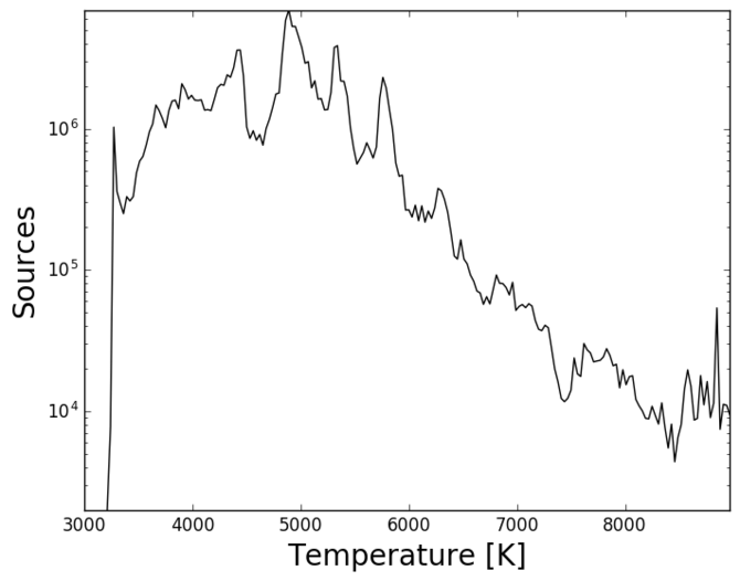
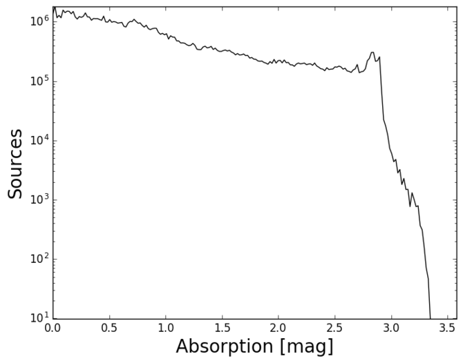
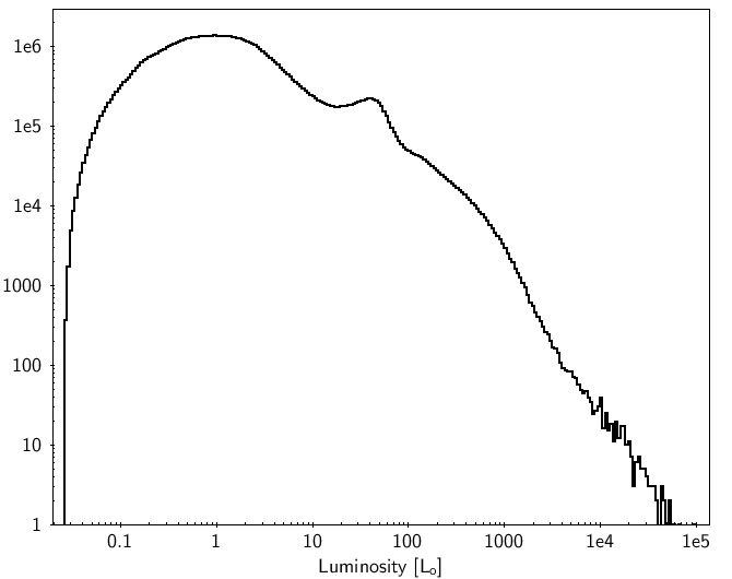
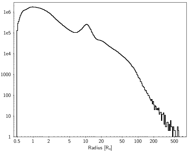
In Figure 10.17, we plot the distribution of the effective temperature, absorption, luminosity and radius (from top left to bottom right) in log scale. The $T_{\mathrm{eff}}$ distribution (top left panel) shows the non-uniformity of the training sample, as already illustrated in Figure 5 of Andrae et al. (2018). $A_{\mathrm{G}}$ (and analogously for $E$($G_{\mathrm{BP}}-G_{\mathrm{RP}}$)) shows a quite uniform distribution with a sharp decrease. We notice that there are no extreme values for luminosities and radii.

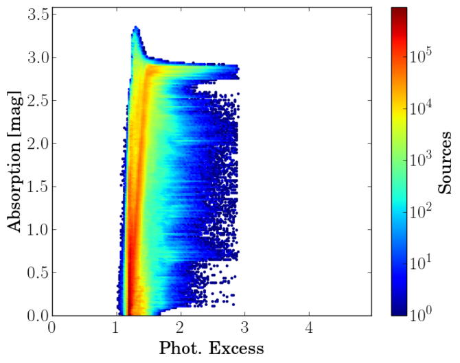
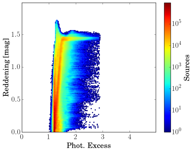
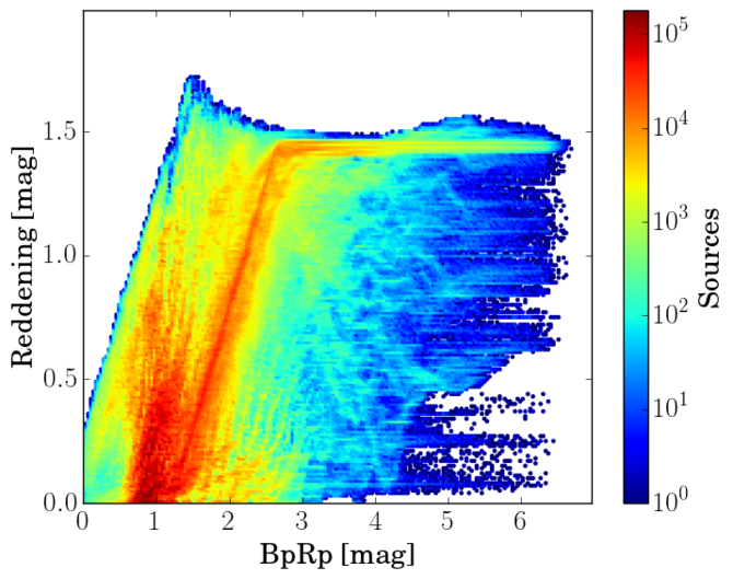
Although the histograms shown Figure 10.17 do not show any significant feature, in Figure 10.18 we plot the relation between Absorption $A_{\mathrm{G}}$, colour excess $E$($G_{\mathrm{BP}}-G_{\mathrm{RP}}$), the photometric excess flux ratio and colour $G_{\mathrm{BP}}-G_{\mathrm{RP}}$. Note that in the left panel, most of the stars with $A_{\mathrm{G}}$$>2.9$ have a low excess flux ratio ( approx.). The same is true in the middle panel, where we plot the colour excess $E$($G_{\mathrm{BP}}-G_{\mathrm{RP}}$) as a function of the photometric excess flux ratio. Again the peak at large extinctions is related to a low excess factor. Analysing further this fact, we see that this feature is also visible when we plot the colour excess $E$($G_{\mathrm{BP}}-G_{\mathrm{RP}}$) as a function on the observed colour $G_{\mathrm{BP}}-G_{\mathrm{RP}}$  (right panel). One would expect a linear tendency, but we observe a horizontal plateau at about $E$($G_{\mathrm{BP}}-G_{\mathrm{RP}}$)=1.4 that extends to red colours.

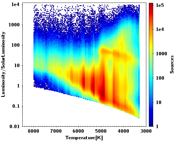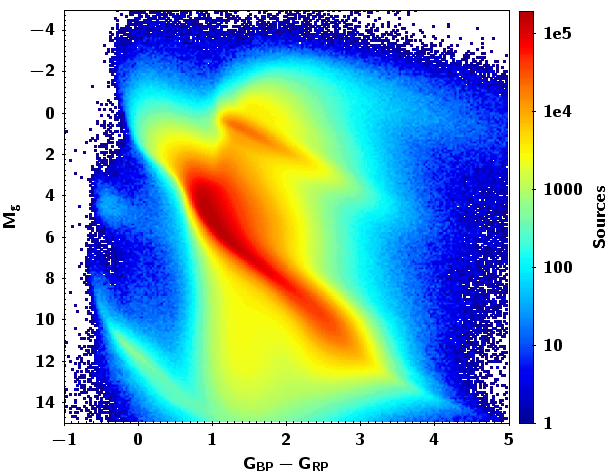
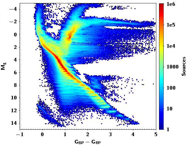
Figure 10.19 shows HR diagrams. In order to compute the absolute magnitude, we use a subsample of the catalog satisfying the quality condition $\varpi /{\sigma }_{\varpi }>5$. The left and middle diagrams show results before and after correcting for absorption and reddening, respectively. Note that when correcting for absorption some discreteness appears when obtaining the absolute magnitude. This is due to the fact that the training set for obtaining absorption is based on a discrete number of absolute magnitudes (Andrae et al. 2018). The last diagram shows luminosity versus $T_{\mathrm{eff}}$, and reveals an unexpectedly large scatter in luminosity for a given temperature, or maybe rather a large scatter in temperature for a given luminosity. About 48% of the sample has luminosities and radii provided. The published uncertainties for the luminosities are below 30%, and for temperatures below 20%. Again, the discreteness in effective temperature comes from the training set, as mentioned above, Andrae et al. (2018).

For a discussion of the astrophysical parameters for duplicated sources see Arenou et al. (2018).

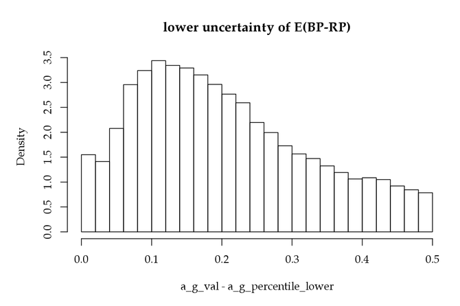
It may be useful to mention problems arising from an incorrect use of extinction and colour excess, in view of their statistical properties. In one of the science demonstration paper accompanying the Gaia DR2, a selection of O-B stars had to be performed to study the young star population. Noting $C_0=(G_{\mathrm{BP}}-G_{\mathrm{RP}})-E(G_{\mathrm{BP}}-G_{\mathrm{RP}})$ the dereddened colour, it would be tempting to select all stars with with, e.g, $C_{\max }=-0.1$. Unfortunately several problems conspire to make such sample mostly representative of stars later than O-B. The first reason originates from the random errors on $C_0$, mostly due to $E(G_{\mathrm{BP}}-G_{\mathrm{RP}})$ (Figure 10.20, left) and to $G_{\mathrm{BP}}-G_{\mathrm{RP}}$ at a smaller extent, and to the non-uniformity of the colour distribution, with a very small fraction of O-B stars in the full population. Even assuming no systematic error on the colour excess, $C_0$ would represent the ${(G_{\mathrm{BP}}-G_{\mathrm{RP}})}_0$ true intrinsic colour convolved by an error distribution; in this case any selection truncating the observed quantity $C_0$ will produce a truncation bias.

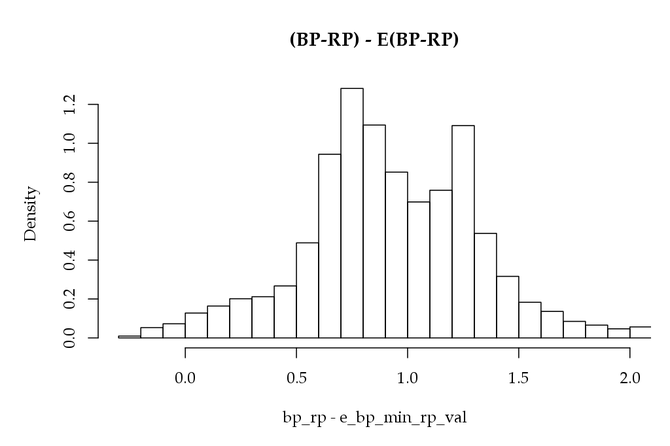
Quantitatively, noting ${\sigma }_C$ the uncertainty of the errors (Figure 10.20, left), that we assume Gaussian for simplification, then the expectation of the true colour given the dereddened one can be computed: $E[{(G_{\mathrm{BP}}-G_{\mathrm{RP}})}_0|C_0]=C_0+{\sigma }_C^2\frac{f^{\prime }(C_0)}{f(C_0)}$, where $f$ is the observed pdf shown Figure 10.20 (right) and $f^{\prime }$ its derivative. Computing the expectation of this from $-\mathrm{\infty }$ to $C_{\max }$ shows a large bias, due to the combination of the steep slope of $f(C_0)$ and of the size of the uncertainty on the colour excess. Moreover, on top of the random errors, the non-negativity of the colour excess unfortunately reinforces this bias.

The net effect has been quantitatively estimated using a sample selection towards the halo, where the extinction is known to be small compared to the random errors of the colour excess; it was found that the sample obtained using contained $24\times$ too many stars, in other terms that most of stars were actually not O-B stars.

In order to improve the sample selection, one may either use stars with the smallest uncertainties only, or rely on external photometry too. This is another example of the biases induced by truncation of noisy data, other examples concerning parallaxes can be found in Luri et al. (2018).