5.3.1 Background Calibration
Author(s): Giorgia Busso
The background signal on the Gaia CCDs collects the contribution of a few components, of different origin:
-
1.
the ‘canonical’ diffuse astrophysical background;
-
2.
stray light from different sources, mostly the Sun but also bright stars, as explained below;
-
3.
two components, related to the CCD electronics, i.e., the dark current signal (dealt with separately) and the charge release (not yet corrected for).
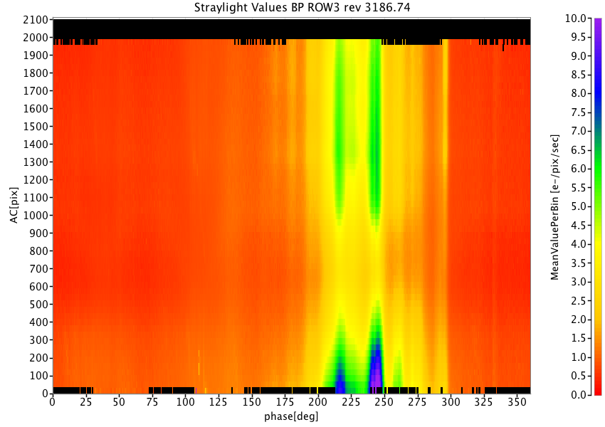
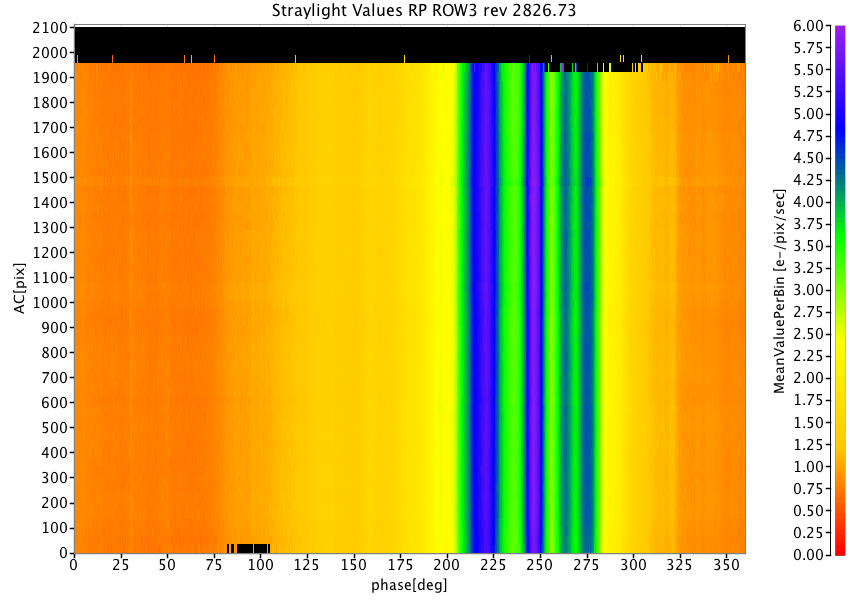
The biggest contribution to the background signal is the straylight, which dominates the other components by a factor which depends not only on the CCD but also on the position inside the same CCD, as evident in Figure 5.5. The worst case is for BP ROW 7 where the straylight can reach values of 27 electron/pixel/second, i.e. more than 100 times the average sky background level of 0.2 electron/pixel/second. See Section 5.3.1 for more details on the straylight correction. The straylight maps however do not correct perfectly for small spatial features, as for instance some peaks, whose size is smaller than the map resolution, or for transient events, as they are calculated by averaging observations on two revolutions. For this reason, an additional correction was applied to the residuals of the straylight in order to obtain a better local background representation (see Section 5.3.1).
Straylight mitigation
The majority of the stray light is caused by the Sun and the strength of this effect depends on the position of the Sun with respect to the satellite. It shows a periodicity corresponding to the satellite spin phase, and a slow evolution in amplitude with the orbital solar distance. Other contributions are in phase with the scanning law, showing contributions from the Ecliptic and Galactic planes.
As a model a discrete map was used, obtained by accumulating two days of observations with distance from the charge injection higher than 100 TDI lines (to avoid the charge release component). There are two types of observations: Virtual Objects (VO, i.e., empty windows acquired for calibration purposes), and science windows for faint stars. For the first one, all samples are used for the background determination. For the second, only the window borders are used, to avoid contamination by the star spectrum. For every transit, the median value on the available samples is computed, to avoid the accidental contribution of cosmic rays, and also the AC coordinate and the heliotropic spin phase (Figure 4.3) are calculated.
The addition of science windows allows a better temporal and spatial resolution for the maps, in comparison with Gaia DR2 when only the VOs were used. The map is built on a grid of 720 bins in the spin direction (one bin is 0.5 degree, previously it was 1 degree bins) and 60 bins in the AC direction (one bin is 35 pixels, corresponding to 6 arcsec, previously it was 98 pixels). All the transits belonging to the same bin are averaged to obtain a median value, to remove outliers. The time validity for a map is 2 revolutions, while in previous releases it was 8 revolutions. This allows to correct for more transient events. Examples of stray light maps are shown in Figure 5.5.
If in the maps there are empty bins, interpolation between the neighbours is performed to fill them. The completed map is then used to build a bicubic spline interpolator which, given the heliotropic spin phase and the AC coordinate of the transit to be corrected, computes the background value in electron/pixel/second. This value is converted to the appropriate one, depending on the window sampling (1D or 2D), and then subtracted from the transit to be corrected.
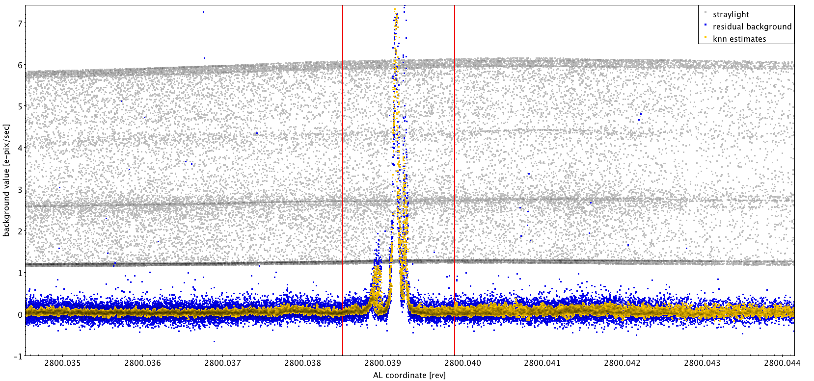
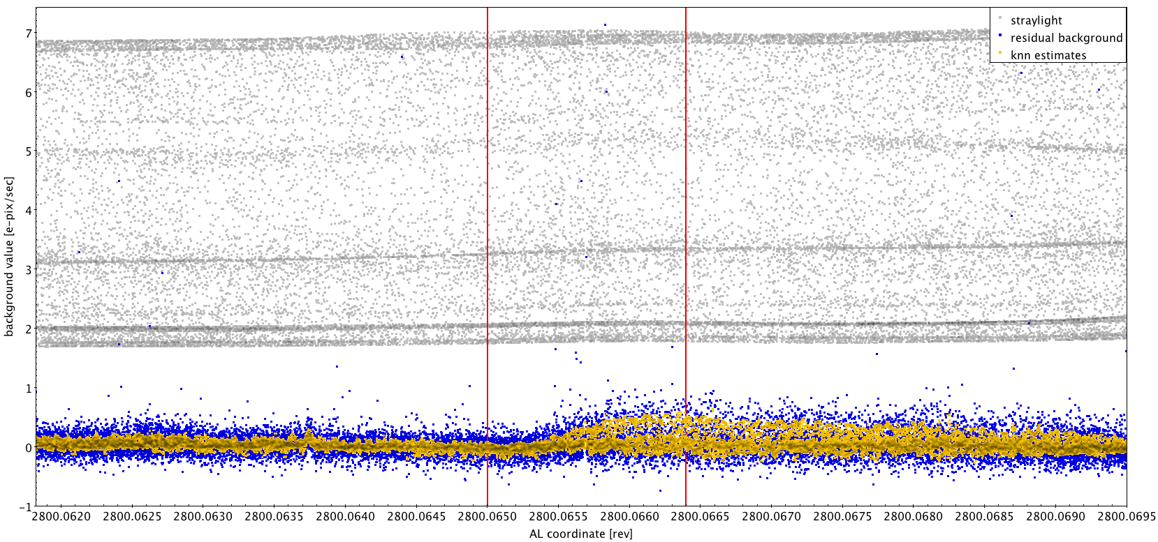
Local background determination
As mentioned in the previous section, the straylight maps are not able to reproduce instantaneous features, such as the narrowest straylight features, spikes from very bright stars or ‘squared’ diffraction patterns. For this reason it was decided to add an additional correction, using a k-nearest neighbours (KNN) algorithm on the residuals of the stray light maps, that is the same data used to build the stray light maps, but with the estimated stray light subtracted. If the straylight map is able to reproduce the correct background value, the residuals should be centered around zero. If there is instead some residual background, the KNN will be able to estimate it. Hence for every transit, the closest 30 residual values were collected and their median was calculated. The value of k=30 is a compromise between having a robust estimate and a contained as possible background value. Figure 5.6 shows some examples.