12.3.6 Redshifts
Redshifts are determined by the QSOC and UGC modules, and stored in the respective qso_candidates and galaxy_candidates tables. Details about the methods used to derive those, as well as specific caveats and limitations of the published redshifts can be found in Section 11.3.14 and Section 11.3.13 respectively, as well as in Delchambre et al. (2023). There is a fundamental difference between the QSOC and UGC results tabulated in the integrated extragalactic tables, in that the UGC redshifts are restricted to those considered eligible by this module (i.e. only redshifts considered as reliable by UGC are published), while the QSOC redshifts are published for any source from the qso_candidates table where such a redshift has been produced. This means that there are many more published QSOC redshifts (6 375 063 sources) than redshifts considered eligible by QSOC (1 834 118 sources). This is essentially due to the fact that QSOC has taken a completeness-oriented approach in its processing, and considered sources with a Combmod quasar probability as low as 0.01 (see Section 11.3.14). As a consequence, the number of sources with an eligible QSOC redshift being labelled as ‘quasar’ (following the ‘Combmod’ class tabulated as classlabel_dsc) is different from the total number of eligible QSOC redshifts (57%). Section 12.5 indicates how to select the sources with the eligible QSOC and UGC redshifts respectively.
Table 12.19 shows the distribution of the ‘Combmod’ classes tabulated as classlabel_dsc among the sources featuring an eligible QSOC and UGC redshift in the respective qso_candidates and galaxy_candidates tables. We remind the reader that the ‘whitedwarf’ and ‘physicalbinary’ classes have a relatively poor purity and in the context of this inventory they can simply be considered as part of the overall ‘star’ sample (see also Section 11.3.2). Owing to its higher purity, the fraction of eligible redshifts labelled as ‘galaxy’ in the UGC sample is significantly higher (99%) than that of the eligible QSOC redshifts labelled as ‘quasar’ quoted above.
| Module | Total | DSC class | |||||
| quasar | galaxy | star | whitedwarf | physicalbinary | unclassified | ||
| QSOC | 1 834 118 | 1 038 955 | 36 305 | 705 506 | 22 727 | 25 925 | 4700 |
| UGC | 1 367 153 | 2458 | 1 350 301 | 13 461 | 15 | 8 | 910 |
Figure 12.15 shows the distribution of these redshifts distribution in the qso_candidates table. The blue histograms correspond to all sources featuring a redshift in this table, while the pink one is restricted to those eligible from QSOC. The other histograms correspond to sources selected by the various modules contributing to the table. Concerning the QSOC sample, a purer selection can be obtained with flags_qsoc = 0, as explained in Section 11.3.14 and Delchambre et al. (2023). Figure 12.16 shows the same distribution for those sources featuring an UGC redshift in the galaxy_candidates table. In the latter, an over-density is observed at redshifts near 0.07. It corresponds to erroneous redshift predictions of bright and close starburst galaxies. See Section 11.3.13 for further details.


The QSOC and UGC respective redshifts can be compared for those sources in common between the two tables, and there are effectively 16,534 sources featuring redshifts from both modules. They are shown in Figure 12.17. Beyond the fact that these two modules do not address redshifts in the same range ([0.08,6.12] for QSOC vs [0.0,0.6] for UGC), some discrepancies appear in particular in case of line mismatch in the QSOC determination (Section 11.3.14). The correlation between the two modules improves when restricting to sources with flags_qsoc = 0, which are expected to have a more reliable redshifts (blue dots). Some QSOC redshifts appear in loci of constant values, and these are believed to arise from erroneous line matches at the edges of the BP/RP spectra, where spurious wiggles are more prominently seen. Conversely, the over-density of UGC redshifts around =0.07 appears as an horizontal population.

A similar comparison is possible against the redshifts inferred from the OA classification. The OA ‘redshifts’ do not strictly correspond to redshift determinations it itself, but instead are derived from the fact that OA classifies QSOs and galaxies in various redshift intervals. The sources classified as such are considered as having redshifts in these intervals, and these are compared to the QSOC and UGC redshifts, as shown in Figure 12.18. As in Figure 12.17, blue dots represent the subset of most reliable QSOC redshifts.


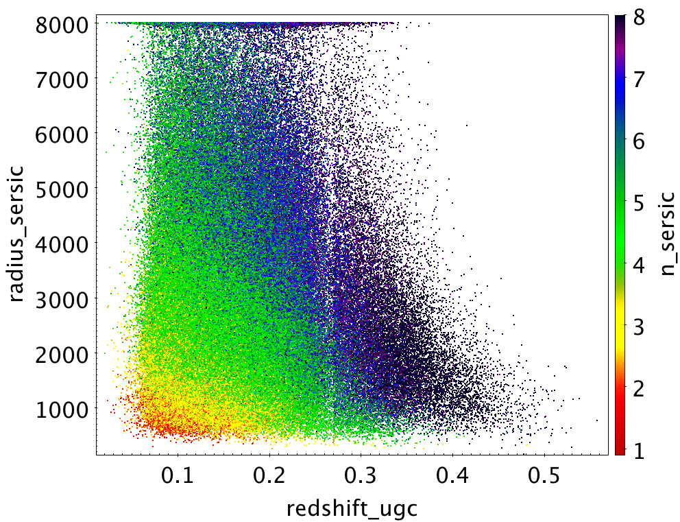
Another way to look at galaxy redshifts is to check their correlation with the radii derived from the various profile fitting of the Surface brightness analysis (Chapter 9). Figure 12.19 shows how the UGC redshift correlates with the galaxy radius derived from the De Vaucouleurs profile fitting in the galaxy_candidates table, showing the expected decrease of radius as the object appears further away. A similar comparison using the Sérsic profile results cannot be done straight-away as the Sérsic radii depend on the Sérsic index. It is, however, possible to check such correlation in intervals of Sérsic indices, as illustrated in Figure 12.20.

 |
 |
A similar check was performed in the qso_candidates table where the QSOC redshift can be compared to the fitted Sérsic radius. No similar correlation is observed, but it should be borne in mind that QSOC was not designed to work on galaxies, and as such poorly predicts the redshift of extended objects.