1.1.3 The spacecraft
Author(s): Jos de Bruijne, Juanma Fleitas, Alcione Mora
Overview
The spacecraft consists of a payload module (PLM; Section 1.1.3) with the instrument and a service module (SVM; Section 1.1.3) with support functions. The prime contractor of Gaia is Airbus Defence and Space (DS), Toulouse, France (formerly known as Astrium). An overview of the spacecraft is provided in Gaia Collaboration et al. (2016).
Payload Module
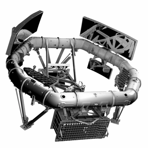
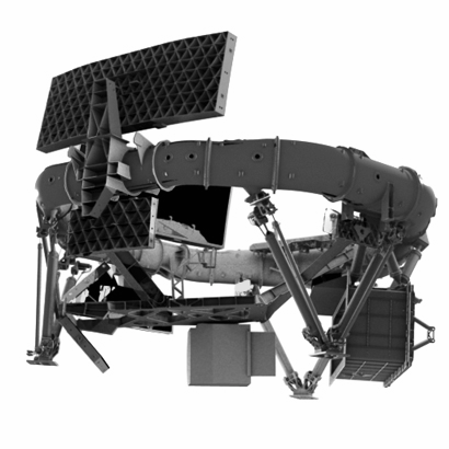
The payload module houses the two telescopes and the focal-plane assembly (FPA; Section 1.1.3). In addition, the payload houses the focal-plane computers (the video-processing units, VPUs, running the video-processing algorithms, VPAs; Section 1.1.3), the detector electronics (PEMs, for proximity electronics modules; Hambly et al. 2018), an atomic master clock (CDU, for clock-distribution unit; Section 1.1.3), metrology systems (basic-angle monitor, BAM, and wave-front sensors, WFSs; Section 1.1.3 and Section 1.1.3), and the payload data-handling unit (PDHU; Section 1.1.3). An overview of the payload module can be found in de Bruijne et al. (2010a) and Gaia Collaboration et al. (2016).
Telescopes
Gaia houses two telescopes, sharing a common focal plane. The lines of sight of the telescopes are separated by the basic angle (). Both telescopes are three-mirror anastigmats with a Korsch off-axis configuration. The entrance pupils are located at the rectangular primary mirrors, and have a dimension of m. A beam combiner at the exit pupil merges the optical paths. Two further flat mirrors in the combined beam fold the light towards the focal plane. The total number of mirrors is hence 10 for both telescopes combined. The image quality of the telescope can be adjusted in flight through (five-degrees-of-freedom) mechanisms attached to the secondary mirrors. An overview of the payload and optical layout is displayed in Figure 1.1. More details on the telescopes are given in Gaia Collaboration et al. (2016).
The focal length of both telescopes is 35 m, providing a plate scale of mas pixel in the along- (AL) and across-scan (AC) directions, respectively.
The focal-plane assembly
The focal-plane assembly (FPA) is shared by both telescopes. It houses 106 charge-coupled-device (CCD) detectors. Since Gaia is continuously scanning around its axis, the CCDs are operated in time-delayed integration (TDI) mode. Gaia’s measurements are very precise in the along-scan direction through precise timing of the signals (line-spread functions, LSFs; see Bastian and Biermann 2005 and Section 1.1.3). In the across-scan direction, the CCD images of most faint stars are binned, substantially reducing the CCD readout noise and science-data volume, with minimum impact on the astrometry. Details on Gaia’s operating principle are provided in Lindegren and Bastian (2010).
The focal plane houses five functionalities:
-
•
metrology (Section 1.1.3 and Section 1.1.3): a basic-angle monitor (BAM) composed of two detectors (one nominal and one cold redundant) continuously measures variations in the basic angle between the two telescopes. Two wave-front sensors (WFSs), with two associated detectors, allow monitoring the optical quality of the telescopes and support refocusing;
-
•
sky mapping (Section 1.1.3): both telescopes have their own sky-mapper (SM) detectors (14 devices in total). These detectors allow detecting objects of interest (point sources as well as slightly extended sources such as asteroids and unresolved galaxies) and rejecting cosmic rays, Solar protons, etc.;
-
•
astrometry (Section 1.1.3): 62 CCDs are devoted to astrometry in the so-called astrometric field (AF);
-
•
spectro-photometry (Section 1.1.3): 14 CCDs are devoted to low-resolution spectro-photometry. Spectra, dispersed along the scan direction, are generated through the use of a blue and a red prism (blue and red photometers, BP and RP);
- •
More details on the focal plane can be found in Gaia Collaboration et al. (2016). The focal-plane layout is shown in Figure 1.2.
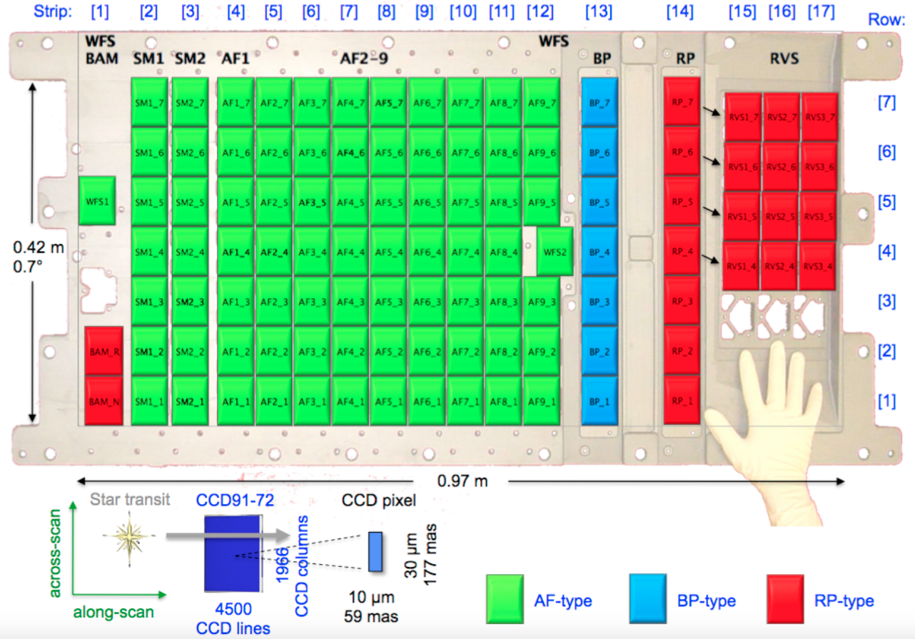
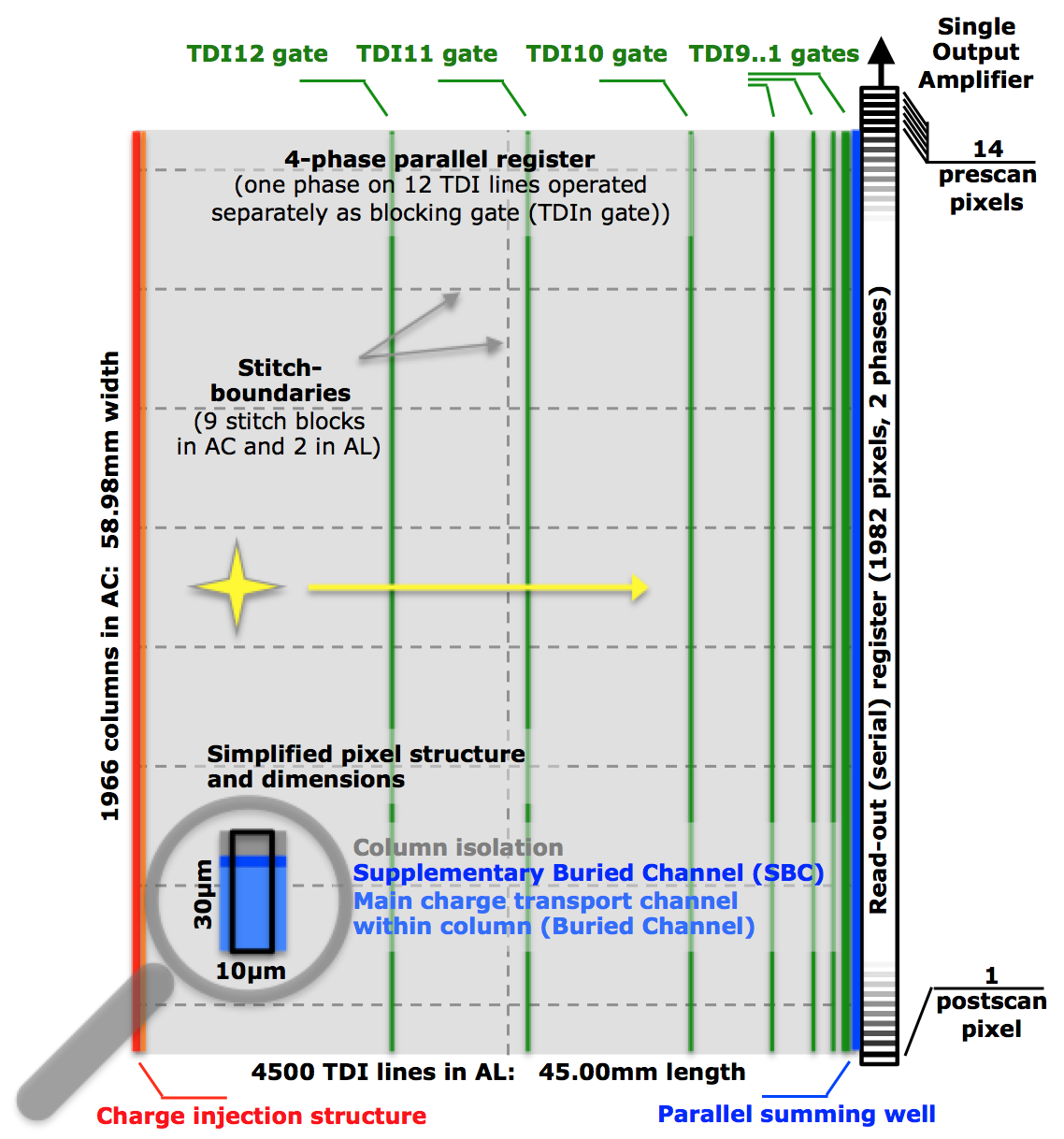
The 106 CCD detectors come in three different types: the broad-band CCD, the blue-enhanced CCD, and the red-enhanced CCD. Each of these types has the same architecture (e.g., number of pixels, TDI gates, read-out register, etc.) but differ in their anti-reflection coating and surface passivation, their thickness, and the resistivity of their silicon wafer. The broad-band and blue CCDs are both 16 m thick and are both manufactured from standard-resistivity silicon; they differ only in their anti-reflection coating, which is optimised for short wavelengths for the blue CCD and optimised to cover a broad bandpass for the broad-band CCD. The red CCD, in contrast, is based on high-resistivity silicon, is 40 m thick, and has an anti-reflection coating optimised for long wavelengths. The broad-band CCD is used in the star mapper (SM), in the astrometric field (AF), and for the wavefront sensor (WFS). The blue CCD is used in the blue photometer (BP). The red CCD is used in the basic-angle monitor (BAM), in the red photometer (RP), and in the radial velocity spectrometer (RVS).
Video-Processing Units and Algorithms
The CCD detectors in the focal plane are commanded by video-processing units (VPUs). Gaia has seven identical VPUs, each one dealing with a dedicated row of CCDs (see Figure 1.2). Each CCD row contains, in order: two SM CCDs (one for each telescope), 9 AF CCDs (except on row 4), 1 BP CCD, 1 RP CCD, and 3 RVS CCDs (the latter only for four of the seven CCD rows). The VPUs run seven identical instances of the video-processing algorithms (VPAs) albeit not necessarily with exactly the same parameter settings. This mix of some hardware and mostly software is responsible for object detection (after local background subtraction), object windowing (see below; see also Section 1.1.3), window-conflict resolution, data binning and prioritisation, science-packet generation, data compression, etc. More details on these functions can be found in Gaia Collaboration et al. (2016).
Detection
The Sky Mapper (SM) CCDs are systematically read in ’full-frame’ mode albeit with on-chip (hardware) binning of pixels into a single sample. The object-detection chains for SM1 (preceding field-of-view) and SM2 (following field-of-view) are functionally identical, but their processing algorithms can be parametrised independently. The detection algorithms scan the images coming from each SM in search for local flux maxima corresponding to celestial objects. A basic data treatment is applied before any on-board processing to correct the raw CCD sample data for gain and offset variations. For each detected local maximum, spatial-frequency filters in both the along- and the across-scan directions are applied to the flux distribution within a samples so-called working window that is centred on the local maximum. Objects failing to meet star-like PSF criteria are classified as prompt-particle event (PPE) or (bright-star) ripple, which means high-frequency or low-frequency outliers, respectively. More details can be found in de Bruijne et al. (2015).
The surviving, star-like detections are classified either as faint detected object or saturated extremity, essentially a bright star. They are sorted by flux and subsequently up to a maximum of 5 objects per TDI line and field-of-view are retained in view of memory-sizing constraints. A list of detected objects is then produced with their attributes, mainly magnitude computed from the flux, observation priority, class of sampling (Table 1.1), type, and along- and across-scan position. Saturated extremities of bright-star wings are matched on-board to produce bright-star detections. Finally, user-controlled Virtual Objects (VOs) are ’artificially’ added to the list of detected objects. Since VOs are propagated across the various CCD detectors in the row controlled by each VPU, they result in empty (sky) windows readout from each device. VOs are used for various calibration purposes (e.g., Section 1.3.3 and Section 1.3.3).
| Instrument | Sampling | Bright mag- | Faint mag- | Window size | Sample size |
| class | nitude limit | nitude limit | (AL AC samples) | (AL AC pixels) | |
| SM | 0 | 5.0 | 13.0 | ||
| SM | 1 | 13.0 | 16.0 | ||
| SM | 2 | 16.0 | 21.0 | ||
| AF1 | 0 | 5.0 | 13.0 | ||
| AF1 | 1 | 13.0 | 16.0 | ||
| AF1 | 2 | 16.0 | 21.0 | ||
| AF2–9 | 0 | 5.0 | 13.0 | ||
| AF2–9 | 1 | 13.0 | 16.0 | ||
| AF2–9 | 2 | 16.0 | 21.0 | ||
| BP/RP | 0A | 5.0 | 11.5 | ||
| BP/RP | 0B | 11.5 | 13.0 | ||
| BP/RP | 1 | 13.0 | 16.0 | ||
| BP/RP | 2 | 16.0 | 21.0 | ||
| RVS | 0 | N/A | 7.0 | ||
| RVS | 1 | 7.0 | 21.0 |
Confirmation
After detection, the available resources for observation in the AF instrument are allocated to the list of SM-detected objects according to their priority (essentially magnitude). Some SM-detected objects may be discarded at this stage due to a lack of resources (’windows’; Section 1.1.3); this is especially true during Galactic-plane scans (GPSs; Section 1.1.5), i.e., periods of time during which the scanning law makes Gaia scan (roughly) along the Galactic plane for several consecutive days. Finally, a filtering stage using AF1 data either confirms objects for observation or discards them if no corresponding signal is observed in AF1.
Astrometric and photometric data
Only confirmed objects with AF1 data are observed in the full AF instrument (AF2–AF9). The observation windows, which are assigned according to the object’s sampling class (Table 1.1), are centred on the object and have an initial rectangular shape. Across-scan sample propagation in each field-of-view, required as a result of the precession of the spin axis, conflict management among windows from different objects, and CCD boundaries, possibly resulting in sample truncation, determine the final window shape and sample size per object.
As the objects reach the end of the AF instrument, similar algorithms as the ones described for AF are triggered for BP/RP. A new resource-allocation process is carried out, for BP and RP independently, optimizing the observations based on the object priority while ensuring a constant number of samples per TDI line. The observation windows, which are assigned according to the sampling class of the object (Table 1.1), are centred on the object and shaped by the field-of-view-dependent across-scan propagation, by window conflicts, and by CCD boundaries in the across-scan direction.
After the SM, AF, and BP/RP raw samples have been collected for an object, they are grouped to form a star packet of type 1 (SP1; Section 2.2.2) and stored in the payload data-handling unit (PDHU; Section 1.1.3). When gathering the raw samples, the VPU temporarily limits the exposure time for bright stars as needed by activating user-defined TDI gates, both in the AF and in the BP/RP CCDs (Figure 1.3 and Table 3.4). SM CCDs are operated with TDI gate number 12 permanently active to avoid excessive saturation from bright stars. Finally, in order to minimise the effect of charge-transfer inefficiency (CTI) due to (native and radiation-induced) charge trapping, a periodic charge injection (CI) is activated in each AF and BP/RP CCD (Section 1.3.3). The shape of the windows is recorded in the SP1-packet header in order to facilitate the window-reconstruction process on-ground (see Fabricius et al. 2016; Section 2.4.3). Each SP1 packet is time stamped with the object acquisition time in AF1. The packet is assigned a File_ID for (prioritised) on-board storage in the PDHU and for down-link prioritisation (Section 1.3.3).
Spectroscopic data
With part of the flux collected from the RP spectrum, an estimate of the magnitude of the object in the RVS instrument is produced. When this is not possible, the RVS magnitude is computed as an extrapolation from the AF magnitude. The object observation priority and class of sampling in RVS (Table 1.1) is derived from this magnitude. A separate resource-allocation process is carried out for the RVS. The observation windows, which are assigned according to the sampling class of the object, are centred on the object and are shaped by the field-of-view-dependent across-scan propagation, window-conflict management, and CCD boundaries.
After the RVS raw samples have been collected for an object, they are grouped to form a star packet of type 2 (SP2; Section 2.2.2) and stored in the PDHU. In RVS CCDs charge injections and TDI gates are not applied (see Cropper et al. 2018 for details). The shape of the RVS windows is recorded in the header of the SP2 packet. Each SP2 packet is time stamped with the object acquisition time in AF1 and the packet is assigned a File_ID for PDHU storage and down-link prioritisation (Section 1.3.3).
Service Interface (SIF) Function
The Service Interface Function (SIF) is a protocol to perform low-level communications with the Gaia payload, in particular the VPUs. It is extremely flexible and hence can have many functionalities. The SIF function is able to read portions (take snapshots) of the VPU random-access memory, while the VPU is nominally operating, and store them in SIF data packets, which are subsequently down-linked to ground. Since the SIF function is versatile and non-invasive, it is not only useful as engineering tool to diagnose and solve problems affecting the VPU, it can also be used to add extra functionality that is not included in the VPU software. The SIF function is frequently used on Gaia, both to provide dumps of VPU-parameter memory blocks in order to validate the (tracking of the) configuration state of the VPU/VPA parameters in the configuration database (CDB; Section 1.2.3 and Section 1.3.3) and to acquire data that come directly from the detector electronics (the proximity-electronics modules, PEMs) and that are temporarily stored in the VPU memory before a fraction of the relevant information is extracted for inclusion in star packets. In this way, the SIF function allows extracting data that is not available in the nominal telemetry, for instance post-scan pixels to monitor radiation damage in the serial (readout) register (Section 1.3.3) or full-frame sky-mapper (SM) images to map selected dense areas (Section 1.1.5).
Payload Data-Handling Unit
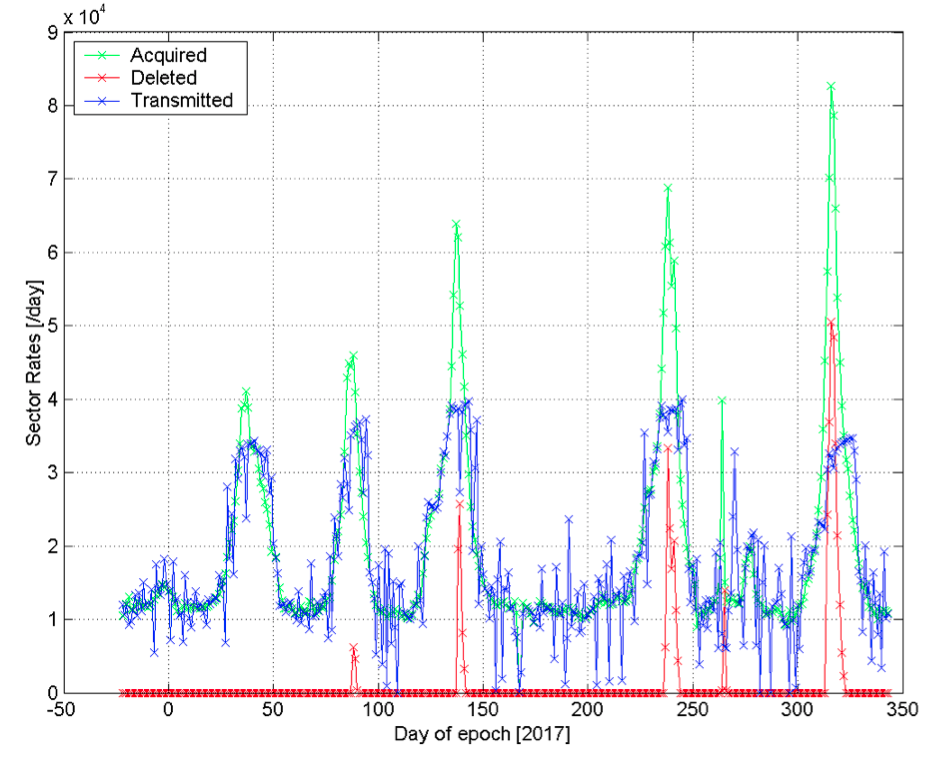
Science / star packets generated on board (Section 1.1.3) are stored in the payload data-handling unit (PDHU) before being down-linked to ground. In order to support user-defined prioritisation of the science telemetry, the PDHU can handle up to 256 different files to store data, each labelled with a unique File_ID. In general, bright stars have a higher down-link priority than faint stars. Under average sky conditions, the PDHU can contain several days worth of science data. When the scanning law makes Gaia scan (roughly) along the Galactic plane for several consecutive days (known as a Galactic-plane scan, GPS; Section 1.1.5), however, the PDHU saturates and a user-defined prioritisation scheme comes in play to govern on-board data deletion (see also Section 1.3.3). This happens a few times per year (Figure 1.4). In general, bright stars have a higher deletion protection than faint stars. More details on the PDHU are provided in Gaia Collaboration et al. (2016).
Clock Distribution Unit
The clocking of all CCD detectors as well as the time tagging of the science data is based on a high-accuracy atomic rubidium clock, embedded in the clock distribution unit (CDU). The CDU contains a rubidium atomic frequency standard (RAFS). This clock is stable to within a few ns over a six-hour spacecraft revolution and has very small temperature, magnetic field, and input voltage sensitivities. The free running onboard time (OBT) counter, which is the time tag of all science data, is generated from the master clock. The spacecraft-elapsed time (SCET) counter in the central data management unit (CDMU), which is used for time tagging housekeeping data and for spacecraft operations, is continuously synchronised to OBT using a pulse-per-second (PPS) mechanism. More details on the CDU are contained in Gaia Collaboration et al. (2016).
Wave-Front Sensor
Two CCDs in the focal plane are equipped with wave-front sensors (WFSs) to enable monitoring the optical quality of the telescopes. The WFSs also allow deriving information to actuate the M2 mirror mechanisms to (re-)align and (re-)focus the telescopes in orbit. The WFSs are of Shack-Hartmann type and sample the output pupil of each telescope with an array of microlenses. The latter focus the light of bright stars transiting the focal plane on the WFS CCDs. Comparison of the stellar spot pattern with the pattern of a built-in calibration source (used during initial tests after launch) and with the pattern of stars acquired after achieving best focus (used afterwards) allows reconstruction of the wave front. See Gaia Collaboration et al. (2016) for details.
Basic-Angle Monitor
Astrometric instrument
The astrometric field (AF) contains 62 CCDs in 9 strips and 7 rows, minus one CCD for the WFS (Section 1.1.3; Figure 1.2). The bandpass of the AF detectors, defining the Gaia band, covers 330–1050 nm; this is mainly set by the telescope transmission in the blue (resulting from the protected-silver coating on the mirrors) and the CCD response in the red. The AF CCDs are not read out in full but only small ’windows’ around objects of interest are read out (Table 1.1; see also Section 2.2.2). The typical window for faint stars is pixels (along-scan across-scan), with the 12 pixels in the across-scan direction typically binned on chip into one single number (the intensity of the along-scan line-spread function, LSF). For bright stars, single-pixel-resolution windows are used, of size pixels (along-scan across-scan; Table 1.1). For more details on the astrometric instrument, see Gaia Collaboration et al. (2016).
Photometric instrument
The photometric instrument contains 2 CCD strips and 7 CCD rows. Half of the CCDs are devoted to the blue photometer (BP, covering 330–680 nm) and the other half are devoted to the red photometer (RP, covering 630–1050 nm). Dispersion of light takes place in the along-scan direction and windows measure pixels (along-scan across-scan; Table 1.1; see also Section 2.2.2). For more details on the photometric instrument, see Gaia Collaboration et al. (2016) and Riello et al. (2018).
Spectroscopic instrument
The spectroscopic instrument contains 12 CCDs in 3 strips and 4 rows. Dispersion of light takes place in the along-scan direction and windows measure pixels (along-scan across-scan; Table 1.1; see also Section 2.2.2). For more details on the spectroscopic instrument, see Gaia Collaboration et al. (2016) and Cropper et al. (2018).
Service Module
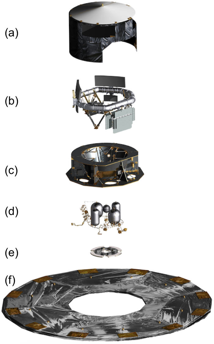
The service module (SVM) supports the payload, both mechanically / structurally and electronically / functionally. A description of the service module can be found in Gaia Collaboration et al. (2016). An exploded view is shown in Figure 1.5.