5.3.6 External calibration
Author(s): Paolo Montegriffo
After the internal calibration has put all the observations onto a common photometric system and the reference fluxes have been computed for all sources, the external calibration effectively provides a means to relate this to other photometric systems and allows for a physical interpretation of the data. This is done providing a response function and an absolute zero point for each pass band. The strategy adopted for the pass band modelling is based on a forward model approach: a response model whose shape depends on a small number of adjustable parameters is fine tuned till the predicted integrated magnitudes fit with the internally calibrated ones for a set of flux calibrators (the SPSS). The model has been designed to reproduce the nominal response curves when all parameters are set to zero. Two different models have been developed: a basic one where the nominal curve is multiplied by a low order polynomial to model possible large scale differences between actual and nominal response (hereafter the Analytic model), and a second one where the nominal curve is summed up with a linear combination of special basis functions derived with Principal Component Analysis (hereafter PCA) to model residuals with the actual filter curve (hereafter the Hybrid model).
Nominal Passband Model
The nominal photonic pass band is modelled as the product of the following quantities:
| (5.8) |
where
-
1.
is the telescope (mirrors) reflectivity;
-
2.
is the attenuation due to rugosity (small-scale variations in smoothness of the surface) and molecular contamination of the mirrors;
-
3.
is the CCD QE;
-
4.
is the prism (fused silica) transmittance curve (including filter coating on their surface) for the BP/RP case.
All these quantities were initially measured by Airbus DS during on-ground laboratory test campaigns. However, the filter wavelength cut-ons and cut-offs in the prism transmittance curves change over the focal plane due to uneven thickness of the prism coating producing bandwidth non uniformity: the expected variation is of about 3 nm in the position of the BP cut-off and of about 2 nm in the position of the RP cut-on (hereafter for convenience only the generic term cut-off will be used for both instruments). Moreover, combining measurements taken all over the focal plane should result in a mean instrument passband with smeared cut-offs. To properly take into account these effects the prism transmittance curve is modelled as follows:
| (5.9) |
where is the tabulated transmittance curve provided by Airbus DS truncated right before and after the cut-off wavelength for the BP and RP case respectively:
| (5.10) |
| (5.11) |
and is a parametric curve based on the Gauss error function and its complementary function:
| (5.12) |
where represents the nominal cut-off wavelength ( nm for BP, nm for RP), and represents the nominal cut-off slope ( for BP, for RP). When the two parameters and are set to zero the nominal transmissivity curve is reproduced to a relative accuracy better than .
Response Analytic Model
The Response Analytic Model represents the mean system photon-counting response function and is the product of the Nominal Passband model with a polynomial function of low degree:
| (5.13) |
This model has been designed to correct for large scale discrepancies between the actual and the nominal response curves, such as those produced by the telescope contamination effect.
Response Hybrid Model
The Response Hybrid Model is an alternative model for the mean system photon-counting response function, and consists of the sum of the Nominal Passband model and a linear combination of special basis functions computed with PCA on a large set of theoretical response curves (hereafter the training set):
| (5.14) |
The training set was built from the extensive set of measurements made by Airbus DS of all the response curve components seen in Eq. (5.8) and available in the DPAC Calibration Data Base (CDB). A MonteCarlo-like procedure was run to apply the relative errors to all measured curves and generate a set of 10,000 different response curves for each pass band. The nominal passband model is then subtracted from these curves, and residuals are arranged in a matrix which is decomposed with Singular Value Decomposition (SVD) into the product of three arrays , where is a diagonal matrix whose elements (singular values) are in non-increasing order, and is an orthonormal matrix whose columns form the orthonormal basis set used in Eq. (5.14). The ordering of singular values ensures that the best approximation of the residuals is achieved for any given number of parameters .
The integrated photometry Instrument Model
Given a source with an energy flux distribution per wavelength unit in units of W nm m, the corresponding predicted mean flux can be modelled as:
| (5.15) |
where is the telescope pupil area in unit of m, is the Planck constant, is the velocity of light in vacuum, and is the mean system photon-counting response function model; in practice, the quantity between brackets represents the source photon flux distribution in units of photons s nm m where is expressed in nm.
Given a set of SPSS, the optimal set of parameters of model to represent the actual photometric system pass band is found by minimising the cost function defined as:
| (5.16) |
where is the Huber loss function defined as:
| (5.17) |
and the variable refers to the weighted residuals for the i SPSS, i.e., the difference between observed and predicted mean flux normalised by the corresponding standard deviation:
| (5.18) |
When the instrument model implies the fit of the response cut-off parameters, as in the BP and RP case, since the model is not linear with respect to the fitting parameters, the minimisation of the cost function is achieved with the Differential Evolution algorithm described by Storn and Price (1997); in all other cases this is obtained by standard linear least squares regression. The usage of the Huber loss function should give intrinsically more robustness against outliers with respect to a traditional -squared loss based algorithm; however, all solvers implement a sigma rejection scheme to under-weight possible outliers in the data.
Solving for the model parameters in the BP/RP case
It can be demonstrated that the integrated magnitudes of the SPSS do not carry enough information to determine the filter cut-off shape with sufficient accuracy, so prior knowledge was needed to constrain the possible variation of the cut-off parameters: the Gaia mean BP and RP spectra could in principle provide such knowledge, however at the time of Gaia DR2 data analysis this kind of information was not yet available, therefore the fitting algorithm was set to allow only for a maximum cut-off shift of 3 nm around the nominal position, according to the Airbus DS findings about the bandwidth variation, as already mentioned in Section 5.3.6. Moreover, the difference between actual and nominal cut-off shapes was expected to be a 2 order correction to the nominal passbands and, in order to avoid as much as possible local minima in the complex cost function space, an iterative fitting scheme was implemented, where:
- •
-
•
the response shape parameters are kept fixed while the cut-off parameters ( and of Eq. (5.8)) are evaluated with the Differential Evolution solver;
The two steps were repeated till convergence was reached.
The , and magnitude scales in the VEGAMAG system
Hereafter we generically use the symbols G and S to indicate respectively the magnitude and the mean system photon-counting response in any of the Gaia , and bands.
The weighted mean flux provided by the internal calibration can be used to define an instrumental magnitude:
| (5.19) |
The Gaia magnitude scale is defined by adding a zero point, , to the instrumental magnitude, as:
| (5.20) |
Traditionally, the value of can be determined by the comparison between the synthetic photometry computed on a set of calibrators with known SEDs and their corresponding instrumental magnitudes: however, since the current passband model has been optimized to reproduce the measured SPSS mean fluxes, the zeropoint computation is simpler. The specific algorithm to compute synthetic photometry depends on the adopted magnitude system: in the Gaia DR2 case, in accordance with Gaia DR1, the photometry is computed in the VEGAMAG system, this being the de-facto standard used internally by the Gaia data processing during the years of preparation of the mission.
The VEGAMAG system is defined so that Vega’s colours are all zero: this is equivalent to normalizing all the observed fluxes to the flux of Vega. The reference spectrum chosen for the Gaia photometric system is a Kurucz/ATLAS9 model (Buser and Kurucz 1992) for the Vega spectrum (CDROM 19) with T = 9550 K, g = 3.95 dex and dex, and v = 2 km s. Its visual magnitude is assumed to be V = 0.0 mag.
Given a source with an energy flux distribution , the integrated energy flux per unit wavelength interval , measured by a photon-counting detector with response , can be expressed as:
| (5.21) |
The synthetic magnitude in the VEGAMAG system is given by:
| (5.22) |
Since all Vega colours by definition are zero, mag. Isolating the zero point from Eq. (5.20) and substituting with the expression in Eq. (5.22), one can set:
| (5.23) | |||||
Using Eq. (5.15) one obtains:
| (5.24) |
Given the passband model optimization described in Section 5.3.6, the expectation value for is 1 and Eq. (5.23) becomes:
| (5.25) |
The error on magnitudes associated to can be computed by propagating the errors on parameters into the above equation. The final uncertainty in the externally calibrated magnitude () in Eq. (5.20)) is
| (5.26) |
where is given by the internal calibration.
Zero point computation in the AB scale
The AB system (Oke and Gunn 1983) is defined in such a way that an object with constant flux per unit frequency interval has zero colour:
| (5.27) |
where is the flux in erg cm s Hz. The constant term is defined to set AB = 0 mag for a source with erg s Hz cm.
Gaia fluxes are expressed in SI units (W m Hz) and hence the value of the constant becomes mag. According to Bessell and Murphy (2012), Eq. 5.27 can be generalised to be used with broad photometric bands:
| (5.28) |
with
| (5.29) |
Using Eq. 5.28 to describe Gaia external magnitudes in the AB system, , and isolating the zero point from Eq. 5.20 one gets:
| (5.30) |
The quantity can be estimated by taking the weighted mean of all the values measured of the SPSS:
| (5.31) |
where
and
being
| (5.32) |
where is computed by propagating the error of the SPSS SEDs ground-based measurements with Eq. 5.21, while is given by the internal calibration.
The standard uncertainty on the weighted mean is computed by using an approximation formula given by Cochran (1977):
| (5.33) | |||||
Summarizing the AB scenario, the externally calibrated magnitude () and its uncertainty () in the AB scale for a source with an internally calibrated mean flux is given by:
| (5.34) | |||||
| (5.35) |
Guidelines to synthetic photometry computations
Gaia DR2 published fluxes are in units of photo-electrons s and are on a arbitrary scale due to the way reference fluxes are defined in the internal calibration process. These fluxes can be converted to meaningful magnitudes by adding the provided zero points in the VEGAMAG or in the AB systems as explained in previous sections. However it is possible to compute synthetic fluxes from theoretical or observed SEDs to be compared with published fluxes in a straightforward way with the following procedure:
-
•
if necessary, convert the SED in units of W nm m;
-
•
transform it into a spectral photon distribution in units of photons s nm m by multiplying for the factor ;
-
•
multiply the photon distribution by the pass band and integrate over the wavelength;
-
•
rescale the integrated flux by the Gaia telescope pupil area ;
The resulting integrated flux is in units of photons s and is in the Gaia DR2 flux scale. Likewise Gaia published fluxes, the conversion to magnitude is trivially obtained by adding the provided zero point to times the of the integrated flux. For a fruitful comparison between Gaia data and 3rd party theoretical or observed data, in order to preserve as much as possible the intrinsic precision of Gaia data we strongly recommend users to forward transform their data to Gaia plane and in particular to work with fluxes in Gaia units: any backward transformation of Gaia fluxes into something else could compromise both its precision and accuracy. For example, the transformation from Gaia fluxes to monochromatic flux densities at some reference wavelength would depend on the source SED which is not available. However if one needs to work with fluxes in physical units this can be achieved using the relations given in the previous section by transforming Gaia DR2 fluxes into AB magnitudes and these to mean and as summarised below:
| (5.36) |
| (5.37) |
hence
| (5.38) |
is the source mean flux per frequency unit in units of W m Hz. This can be converted to the mean flux per wavelength units in units of W m nm as follows:
| (5.39) |
where is the pivot wavelength defined as
| (5.40) |
Finally the mean energy flux can be converted to the mean photon flux:
| (5.41) |
where
| (5.42) |
accordingly to Bessell and Murphy (2012) is the mean photon wavelength of the passband. Mean photon wavelengths and pivot wavelengths are give below in Table 5.4. Other commonly used wavelengths associated with passbands like the isophotal wavelength or the effective wavelengths depend explicitly on the source spectral energy distribution and hence are not computed here.
Results
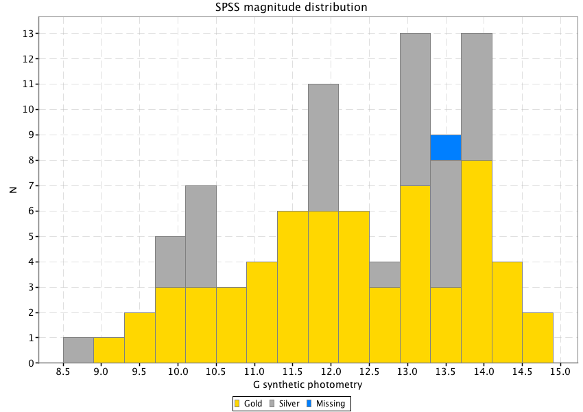
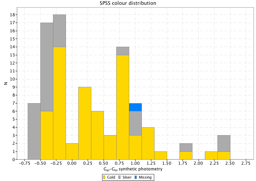
The data exported from internal calibration which matched the SPSS IDs consisted of 93 records out of the 94 sources present in the V1 SPSS list (one star was missed by the cross-match identification process because of its high proper motion): a set of 64 SPSS were extracted from the gold sources (i.e. sources with colour in the range, where the time link-calibration could be applied, see Section 5.4.3) set while the remaining 29 were recovered from the silver set sources (i.e. sources with colour outside the range, where an ad hoc calibration had to be applied, see Section 5.4.3). The distribution of collected data as a function of the nominal magnitude and colour is shown in Figure 5.7.
To provide a visual comparison between the Gaia DR2 photometric system properties and the pre-launch nominal one, we show in Figure 5.8 the difference between synthetic and instrumental magnitudes as a function of the colour for the 93 SPSS: while the magnitudes are comparable with internally calibrated photometry, the data exhibit a complex behaviour and clearly show a rather strong colour term for sources bluer than mag. This colour term is presumably due to the combination of internal calibrators colour selection with time link calibrations to correct for telescopes transmissivity variations due to contamination. The case shows a clear colour term with redder sources being fainter than expected.
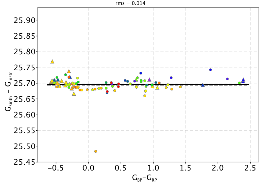
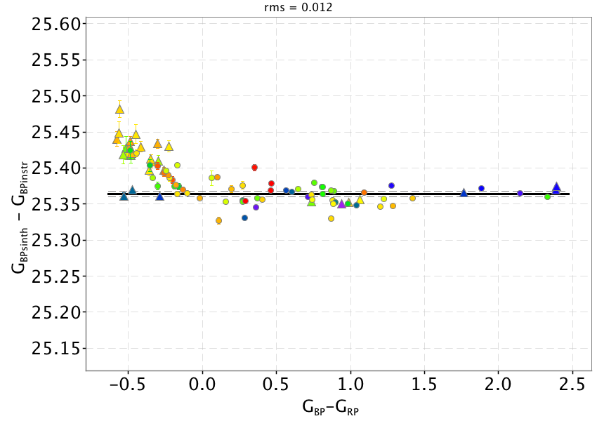
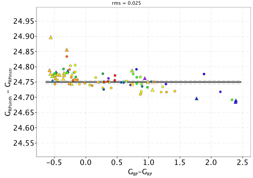
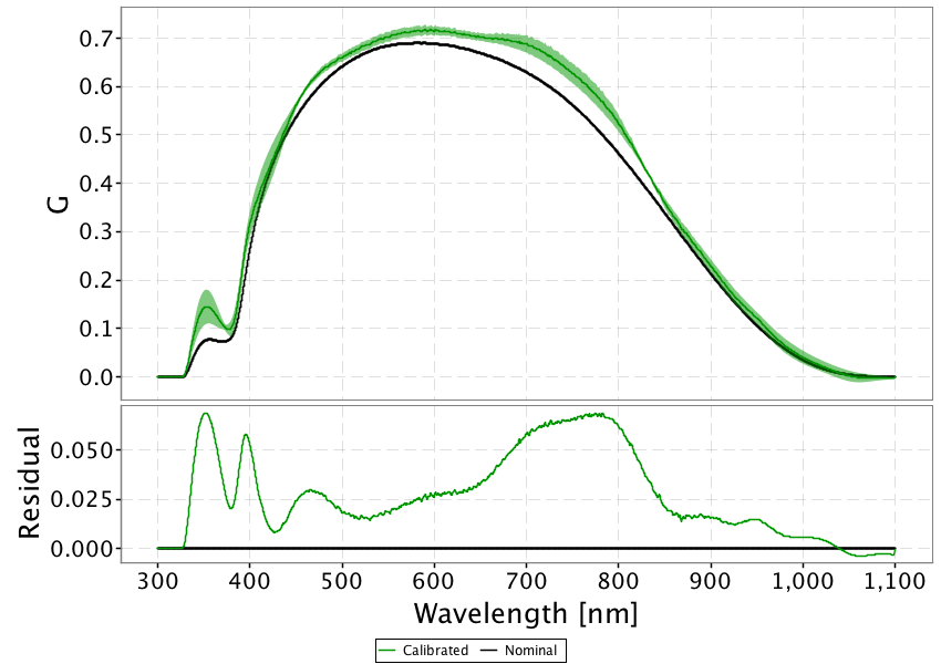
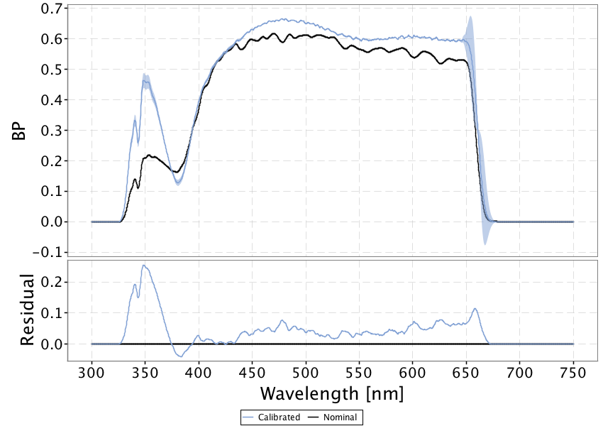
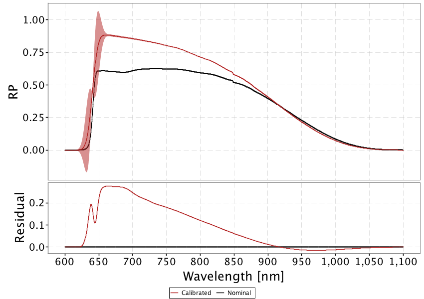
Figure 5.9 shows the calibrated Gaia pass bands for the G, and photometric systems; each curve is compared against the nominal counterpart and the level is represented as a shaded region. The G and curves have been modelled by the Response Hybrid Model using respectively 4 and 3 basis functions. The curve exhibits a pronounced bump in the blue side with respect to the nominal curve, that is needed to correct for the colour term left into the silver sources data by the Time Link Calibration. The case was more problematic to optimize, because the output curve resulting from the Hybrid Response Model had an implausible shape independently of the number of basis function used: this is an evidence that the actual pass band shape is significantly different from the nominal one and the PCA based representation fails to give an acceptable result. For this reason a 1 degree polynomial function was used for the Analytic Response Model of the .
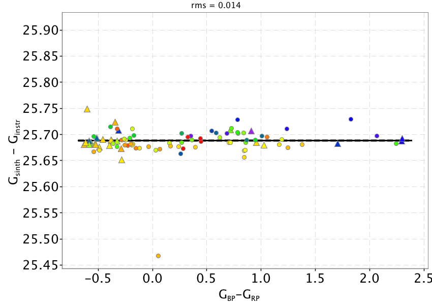
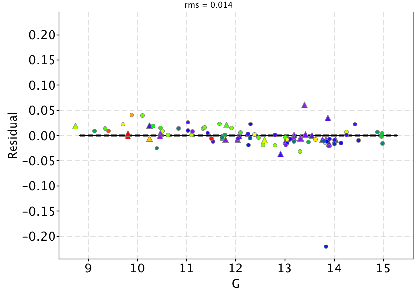
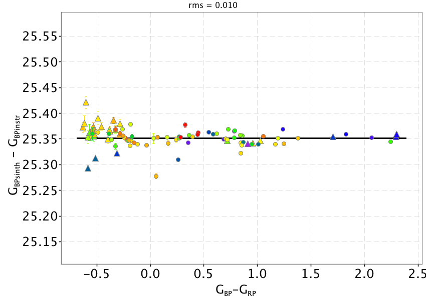
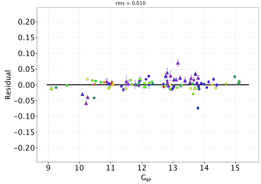
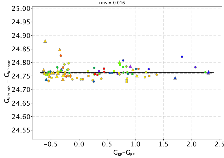
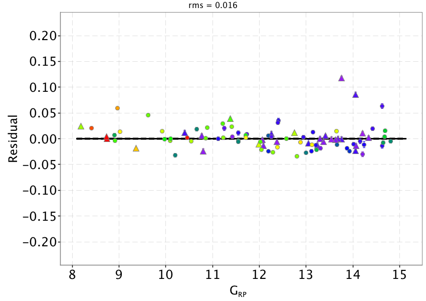
Once the calibrated pass bands are used to recompute synthetic photometry, the comparison with SPSS mean fluxes shows that the colour terms are effectively removed (Figure 5.10 top panels). The solid black lines represent the derived external calibration zero points which are given in Table 5.2.
| Band | ZP | error |
| 25.6884 | 0.0018 | |
| 25.3514 | 0.0014 | |
| 24.7619 | 0.0019 |
These passbands were released for internal DPAC use in July 2017 and adopted in the photometric processing to calibrate the magnitudes to be released in Gaia DR2. These passbands are available to be downloaded at the following url: https://www.cosmos.esa.int/documents/29201/1645651/GaiaDR2_Passbands_ZeroPoints.zip.
A following analysis showed that the BP/RP spectra were better described by taking into account an offset in the RP cutoff wavelength position. A new set of revised passbands was then derived in October 2017 to introduce this and a few other minor changes. These updated passbands can be downloaded at the following url: https://www.cosmos.esa.int/documents/29201/1645651/GaiaDR2_Revised_Passbands_ZeroPoints.zip.
The left panels of Figure 5.10 show residuals with respect to the adopted zeropoint as function of , and magnitudes respectively to investigate for possible systematics left by the internal calibration. The only appreciable effect is visible in the case, where sources with mag seem to have slightly higher residuals with respect to fainter sources.
Finally, Table 5.3 gives the zeropoints for the three passbands in the AB system: these values can be used to convert Gaia photometry to the AB system.
| Band | ZP | error |
| 25.7934 | 0.0018 | |
| 25.3806 | 0.0014 | |
| 25.1161 | 0.0019 |
| Band | [nm] | [nm] |
| 640.50 | 623.06 | |
| 513.11 | 505.15 | |
| 777.76 | 772.62 |