4.4.3 Astrometric processing
Author(s): Thierry Pauwels, Federica Spoto, Paolo Tanga
Basic processing
The basic processing of the Astrometric Reduction module followed the same procedure as IDT, and consisted of three consecutive coordinate transformations.
At input, coordinates were given in the WRS (Window Reference System), and consisted of pixel coordinates of the SSO inside the transmitted window along with timings in OBMT, the internal time scale of Gaia (Gaia Collaboration et al. 2016). The origin of the WRS was in the reference pixel of the transmitted window. For the transmitted window the coordinates in pixels of the window, and the binning strategy were given. The timings in OBMT corresponded to the time of read-out of the reference pixel of the transmitted window.
The first step of the astrometric data reduction was to compute the epoch of observation, technically the timing of crossing of the fiducial line, i.e., the centre line of the exposure on the CCD. This is half the exposure time earlier than the reference time, plus a correction for the exact location of the photocentre of the SSO in the transmitted window, and a correction for the size of the transmitted window. The exposure time itself was only dependent on the gating strategy for the window (Gaia Collaboration et al. 2016). Note that due to the TDI mode of Gaia the epoch of observation in TDI steps was equal to the AL coordinate of the SSO on the observed strip along the sky, such that position and timings were not independent quantities.
The second step was a conversion from the WRS to the SRS (Scanning Reference System). In this latter system the coordinates are angles parallel and perpendicular to the scanning direction of Gaia, and the origin of the coordinate system was in the centre of the focal plane of Gaia. The coordinate transformation included the geometric calibration, describing the difference between the nominal and the real positions of the CCDs in the focal plane of Gaia.
The third step was a conversion from the SRS to the CoMRS (Centre-of-Mass Reference System), a non-rotating coordinate system with origin in the centre of mass of Gaia.
The last step was a conversion from the CoMRS to the BCRS (Barycentric Reference System), with origin in the barycenter of the solar system. This last transformation gave the right ascension and declination of the SSO, i.e., the direction of the unit vector from the centre of mass of Gaia to the SSO. It included the correction of the light aberration with its relativistic component, thus eliminating any contribution from the relative motion.
In the course of these coordinate transformations, timings were converted from OBMT to TCB(Gaia).
This procedure was the same as the procedure applied for stars by IDT, and the reader is referred to Chapter 3 for the full details.
Positions
Positions were given as right ascension and declination in the BCRS reference frame. This is the direction of the unit vector from Gaia to the photocentre of the SSO. No correction for the light travel time from the SSO to Gaia was applied.
The most important limitation of the processing adopted for Gaia DR2 derives from taking into account the light bending by the solar gravity field (including contributions from the Sun, Earth and Jupiter), which was computed with the same approach used for the stars. However, since the origin of the light, i.e. the SSO, is inside the Solar System, the path of the light beam reaching the observer does not travel through the whole solar gravity field, as for stars. The absolute difference can be up to 2 mas at solar elongations 90 degrees (median: 1.2 mas). A correction should be applied by the users of these data if the ultimate precision is expected. This limitation will disappear in forthcoming releases.
Other corrections of the astrometry, depending on SSO physical properties such as size, shape and scattering properties were not applied at this stage. This include in particular corrections of the position of the photocentre with respect to the centre-of-mass.
At each transit, at most 9 positions were given, corresponding to the AF CCDs: AF1 through AF9. SM CCDs were intended to be processed as well, but the validation showed already at an early stage that positions derived from the SM CCDs have errors much larger than the formal uncertainties resulting from the processing.
Therefore, SM positions were systematically rejected right at the start of the processing. Although for the vast majority of the transits, observed using 1-D windows, the SM CCDs would be the only source of information about the AC component of the position of the SSO, the AL components of the positions were sufficient to compute an orbit, as shown by the validation process. In many cases, however, there were less than 9 positions in a transit. There are several reasons for this:
-
1.
Row 4 contains only 8 AF CCDs, rather than 9, so any transit through row 4, can contain no more than 8 positions.
-
2.
The software failed to produce a good position for a particular CCD, such as the proximity of a star or a cosmic ray signal.
-
3.
A position may have been found to be of too low quality and rejected.
-
4.
The transmitted window is always propagated on-board from the SM CCD to the AF CCD assuming the image to be that of a star. The proper motion of the SSO in the course of a transit may, however, cause the SSO to leave the transmitted window before the end of the transit. As a result, after the first CCDs, the SSO can exit from the window.
The last effect is the most complex. Often, in the last CCD in which the SSO is still detected, a substantial fraction of the flux falls already outside the window, causing the photocentre to be shifted towards the centre of the window. In such cases the last position has also been removed from the output. See Figure 4.18 for an example.
When plotted on a sky map in a right ascension–declination coordinate system, the different positions of a transit of an SSO do not align, and at first sight it may look that the SSO has a zigzag motion for the duration of a transit (roughly 40 seconds). However, this is an artefact of the observing procedure, and by taking into account the correct error ellipse, one finds that the given positions are perfectly compatible with a linear motion. The apparent zigzag motion is a consequence of the on-board observing and binning strategy of Gaia. In the SM CCD the object is detected, and a transmitted window is defined, centred on the object. This window is propagated from the SM CCD to all AF CCDs, taking into account the precession of the satellite, but not the motion of the SSO. The precession can induce a shift of the transmitted window in AC direction of up to 4 pixels from one CCD to the next. The exact value, of course, does not correspond to an integer number of pixels, but the windows must be aligned on an integer pixel. The shift from one CCD to the next one may thus alternate between different values. Since in the AC direction, in the case of 1-D windows, we have no other information on the position, but that the SSO is inside the window, the zigzag motion reflects only the AC displacement of the transmitted windows on the different CCDs and not the motion of the SSO.
Figure 4.18 shows most features of the positions and their uncertainties. The figure covers a portion of the sky with an area of 400 400 mas. The horizontal axis is aligned with right ascension and the vertical axis with declination. The black arrow represents the scanning direction of Gaia, parallel to the AL axis. The large coloured dots represent the positions as published in the catalogue, while the scattered dots sample the uncertainty ranges on the positions. Uncertainties are very small in the AL direction, and very large in a direction perpendicular to it. The red line connecting the different positions of the transit shows the apparent zigzag motion of the SSO. This apparent zigzag motion is entirely due to the uncertainty on the position perpendicular to the AL direction and the way the transmitted windows are assigned, and is not real. The black line with the coloured squares represents the fit of a linear motion, and one can see that a linear motion fits perfectly the positions AF1–AF6. In interpreting this fit, one has to keep in mind that only the AL component of the velocity of the objects is real. Careful inspection of the plot shows that AF7 does not fit the linear motion any longer, probably because part of the signal fell outside the transmitted window. In AF9, the SSO is likely completely outside the transmitted window, and the processing fails to derive a corresponding position. In this case, the AF7, AF8 and AF9 positions were rejected, and only the AF1–AF6 positions have been published.
Timings
Timings were given in TCB(Gaia), which is the primary time scale for Gaia. Timings correspond to mid-exposure, or more technically, to the instant of crossing of the fiducial line on the CCD by the photocentre of the SSO image. The exact location of the fiducial line depends on the gating strategy applied for that particular window. This gating strategy corresponds to the exposure time. See Gaia Collaboration et al. (2016) for a detailed explanation of the gating strategy.
As a convenience for the user, timings were also converted to UTC, as explained in Gaia Collaboration et al. (2016). UTC is, however, not strictly defined, and for high-precision computations, users should not use UTC timings.
The uncertainty on the timings is given as 1 TDI cycle, which corresponds roughly to 1 ms. More precise timings would require a detailed modelling of the transfer of the charges in the CCDs but in practice this was not needed. A typical main-belt asteroid moves at most 10–20 as during one TDI cycle, which is much less than the uncertainty on the best position. Fast moving objects (e.g. NEOs) may move substantially more during one TDI cycle, but smearing of the image during the 4-second exposure dominate the astrometric uncertainty. Therefore, limiting the precision of the timings to 1 TDI cycle is quite justified.
Observing an SSO by Gaia is considered to be a local Gaia event. Consequently, the timings given were the timings of arriving at Gaia of the light reflected by the SSO. In Gaia DR2 no information has been given about the light time correction, i.e. the epoch of sunlight scattering by the SSO surface.
Filtering
Filtering was a very important activity of the Astrometric Reduction processing. It ensured that positions that do not really belonged to an SSO were rejected, as well as positions that did not meet high quality standards. Filtering has been applied both at the level of individual positions (individual CCDs), and at the level of complete transits. Many parameters of the filtering were adjusted by hand, by carefully checking how the software was behaving when treating data about well-known asteroids, and the parameters were optimized to have a minimal number of both false positives and false negatives, i.e., so as to reject a maximum number of bad detections, while minimizing the number of rejected genuine good positions. Needless to say, when treating very large numbers of objects in an automatic way, it is inevitable that the data will contain some false positives. In practice, many circumstances are encountered that require an efficient rejection filter. They are listed in what follows.
No data at input
When the astrometric reduction module received data from the centroiding module, already some positions were missing. These are CCD where the centroiding module failed to fit a PSF or LSF to the image. These positions have obviously been filtered out.
Weird cases
Some weird cases were too difficult to treat or could give rise to positions of which the precision could not be guaranteed. These positions were rejected right at the start of the processing. They included:
-
•
all positions from the SM CCDs
-
•
any position with a truncated window
-
•
any position suspected to be contaminated by a nearby star
-
•
any position that had all samples to zero
-
•
any position that had eliminated samples
-
•
any position that was affected by an AOCS update
-
•
any position that was affected by a non-nominal gating
-
•
any position that was too close to the celestial pole.
All situations in the list above were reported by upstream processes, and interested users should refer to the appropriate sections of this document for more details.
Moreover, some transits were flagged as being problems as a whole. In such cases, the complete transit with all its positions was rejected. These included:
-
•
all transits with truncated windows.
These cases were also reported by upstream processes.
Error-magnitude relation
When analyzing the relation between the AL uncertainties coming from the centroiding process and the magnitude for confirmed real detections of SSOs, they all lie between rather tight limits. Positions with reported uncertainties unrealistically large or small for the given magnitude were clearly not detections of the SSOs. This was used to define a first, very simple selection criterion. After careful investigation, we defined the following conditions:
| (4.5) |
where is the AL component of the computed uncertainty from the centroiding, and where and are the corresponding minimum and maximum allowed values, given by:
| (4.6) |
| (4.7) |
where is the magnitude available at the step of astrometric processing (a preliminary value computed from IDU, the quality of whom is sufficient for our goals). All positions not satisfying relation (4.5) were rejected.
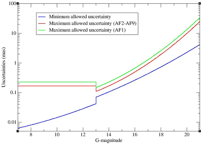
Figure 4.19 shows the relation defined by Equation 4.5. Magnitude 13 is the transition between 1D and 2D windows. For brighter SSOs the uncertainties are no longer expected to get smaller because of the gating strategy, i.e. brighter objects get shorter exposure times. AF1 has been found empirically to have systematically slightly larger uncertainties. Therefore uncertainties for AF1 were allowed to be 1.35 times larger than for other CCDs.
Fitting a linear motion
The displacement of an SSO on the sky in the course of a single FOV transit can be assimilated to a linear motion. Even for extremely close and fast objects, after using a gnomonic projection on a plane tangential to the sky, the motion will be linear, with both space coordinates being linear functions of time. A very efficient way to remove wrong detections, was to check the linearity of the motion, and whether all positions fitted on the regression line within the computed uncertainties. This way, we could efficiently reject detections for which part of the flux falls outside the transmitted window, causing the position to be shifted to the window centre.
The adopted procedure was as follows. First, a linear regression of the positions as a function of epoch was computed, taking into account the proper weights resulting from the uncertainties. In this process, the SM position had already been removed. Whenever the complete set of positions was found to be consistent, meaning that all residuals on this fit were smaller than a given threshold, the transit with all its positions was accepted. If at least one residual was found to be too large, then an iterative process was started, where in the first iteration one position is removed from the transit, and in each iteration one more position is removed until a minimal set is reached. The minimal number of positions in a transit to check for consistency is user selectable, but cannot be lower than 3, since any set of only two positions will be consistent with a linear motion.
In the th iteration the software tries all possible combinations of the transit with positions removed. If it finds one single combination to be a consistent set, the transit will be accepted, but the positions that had to be removed to get the consistent set are considered as outliers, and are rejected. If for all the sets, none is found to be consistent, meaning there is still at least one residual which is too large, this means that no linear motion can be found with positions removed, or that at least positions are bad. A next iteration is then started with positions rejected. If, however, more than one set of positions is found in the -th iteration to be consistent, the software cannot decide which positions are the outliers to be rejected. The threshold is then relaxed, and the whole procedure is repeated starting with all positions, and gradually removing more and more positions from the transit, until either a single set is found to be consistent (but now using the relaxed threshold), in which case the transit is accepted with the positions rejected to get the consistent set; or until more than one consistent set is found with the same number of positions removed, in which case the threshold is again relaxed, until a maximum value of the threshold is reached.
If the maximum value of the threshold is reached, and there is still more than one consistent set with the same number of positions, the transit is considered to be of low quality, and is rejected as a whole. If the transit at the start contains less than the minimal number of positions to search for consistent sets (e.g. because the SSO was so fast that it left the transmitted window after two CCDs, and that this caused already all other positions to be rejected on the basis of the error-magnitude relation), the complete transit is accepted, without any position being rejected. This means that the consistency check is in fact by-passed. If, however, the procedure reaches the minimal number of positions to search for consistent sets without finding any, the transit is considered not to belong to an SSO, and the complete transit is rejected.
For Gaia DR2 the following parameters have been set:
-
•
Threshold for the residual: 2 sigma, meaning that residuals considered as 2-D vectors, should not extend further than twice the error ellipse.
-
•
Maximum relaxed threshold for the residual: 4 sigma.
-
•
Increment to relax the threshold: 0.1 sigma.
-
•
Minimum number of positions in a consistent sets: 3, i.e. at least 4 positions are required to be able to identify an outlier.
Minimum number of positions in a transit
After applying all the other filters, a final check was to assess how many positions are left in a transit. Since the search of consistent positions cannot be performed with less than three positions, it is dangerous to accept transits with less than three positions. The minimum number of positions left in a transit is user selectable and any transit left with less than this number of positions was rejected as a whole. For Gaia DR2, however, with an a priori list of transits to be processed, that were already identified as belonging to SSOs, and with a further quality check downstream by fitting an orbit to the positions, it was found safe to set this limit to 2. Extensive checks have shown that the vast majority of the transits with only two positions are good positions that belong to real SSO. This means that only transits with one single position left have been rejected.
Magnitude limit
Transits brighter than 10 were found to show problems with the positions. s with an orbit turned out to be substantially larger than the computed uncertainties. For instance, in the case of the dwarf-planet (1) Ceres, the s turned out to be larger than expected by a factor of 5. The reason of this discrepancy is under investigation, but it is clear that SSOs of large apparent size and high brightness fall well outside the optimized range of performance of Gaia. While corrections have been studied and will be tested for future releases, in Gaia DR2 all objects that reach have been eliminated.