4.2.1 Selection of objects for Astrometry and Photometry

Author(s): François Mignard, Laurent Galluccio

For the Gaia DR2 the SSO processing was carried out for an off-line selection of targets instead of activating the automatic recognition that will be used at a later stage. This had the advantage of limiting the volume of data entering the pipeline and offering a near certainty that only genuine SSOs were selected. This simplification was considered desirable for the first mass processing of solar-system sources over a relatively short time span. To this aim a list of transit identifiers associated to the passages of known SSOs was generated by a pre-processor and this list was added to the input data ingested by the processing chain. Several criteria were applied to select a valuable subset of objects.

• •

  We aimed at having between 10 000 and 15 000 SSOs.

• •

  Representatives of all the broad categories of asteroids were sought (NEAs, MBAs, Trojans, etc.).

• •

  No transit of an object should be lost because its apparent magnitude was becoming too faint at small solar elongation, when the distance to Gaia was the largest.

• •

  A planetary transit was not selected if a star, another SSO or a contaminant generated by a bright star was found too close to the object during its observation by Gaia.

• •

  Each selected SSO had to have been observed at least 12 times over the 22 months covered by the Gaia DR2 data.

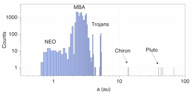
These conditions were applied iteratively until a satisfactory selection meeting all the requirements was achieved. The final input selection had $\mathrm{318\hspace{0.17em}290}$ transits for $\mathrm{14\hspace{0.17em}125}$ SSOs. The coverage in orbital semi-major axis displayed in Figure 4.6 shows that SSOs within of each of the broad categories are found in the selection.

The list has been created in three main steps:

• •

  Prediction of all the possible transits for a set of SSOs over the Gaia DR2 time span using the Gaia orbit, the scanning law and a numerical integration of the SSO motion starting from the osculating elements and osculating epoch given in the Astorb data (see Section 4.4.1).

• •

  Cross-matching the transits with the Gaia IDT detection to ensure that a potential candidate SSO had been actually seen by Gaia and observed during the predicted transit.

• •

  Iterative filtering on the tentative list to ensure that the selection criteria were met and no contaminant was left.

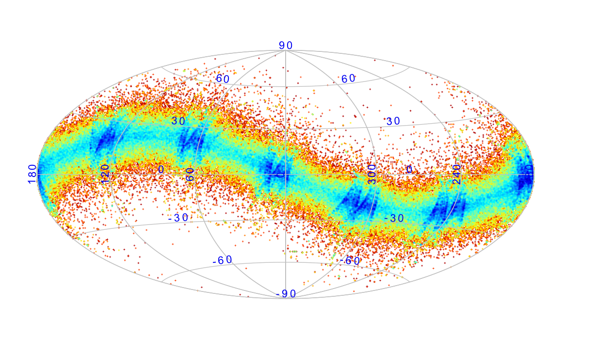
The sky distribution of the selected observations is shown in Figure 4.7 on a density plot in equatorial coordinates. The SSOs are all found in the vicinity of the ecliptic plane, but the distribution in longitude is markedly non uniform with periodic features of higher (deep blue) and lower concentration. This is a known artefact resulting from the Gaia scanning over a relatively short duration of 22 months compared to the nominal mission of five years. The features seen every 60 ${}^{\circ }$ shift of 72 ${}^{\circ }$ every year, so that the coverage becomes nearly uniform after five years.

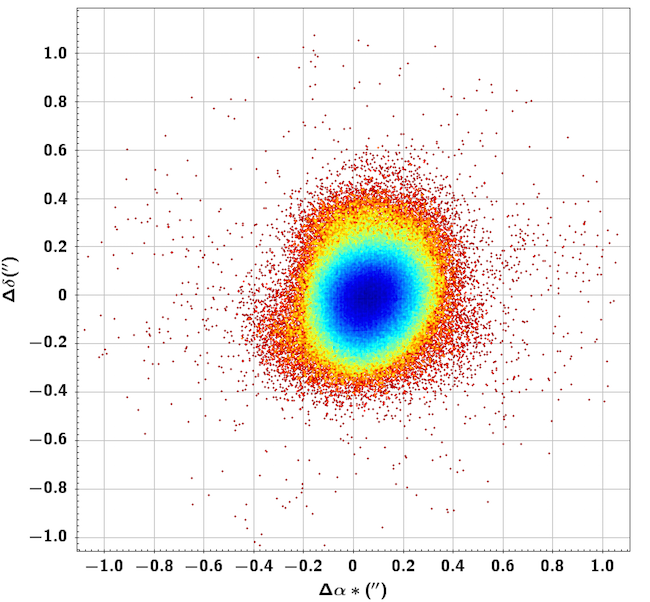
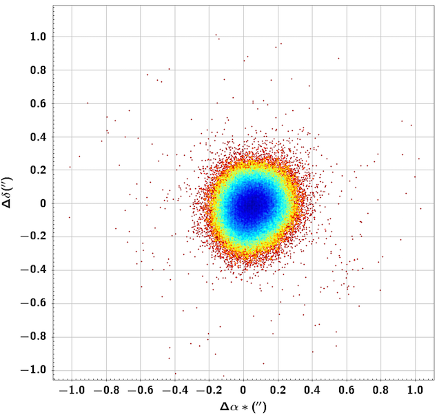
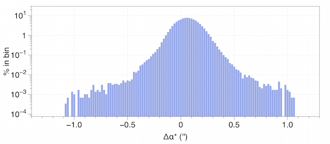
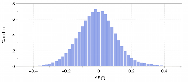
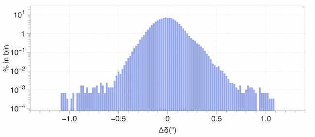
Besides the orbital elements, the main features of the selection procedure are shown in the set of separate plots. The scatter distribution between the computed position and the IDT solution is shown in Figure 4.8, with the data from October 2014 to May 2016 (left) and from October 2015 to May 2016 (right) being shown separately. IDT data from the transition scanning law (NSL-Smooth) in September 2014 are very poor and not included in this analysis. These are density plots and the concentration is essentially within $\pm 0.2$ ${}^{\mathrm{\prime \prime }}$($>95\%$ of the data set). The distribution is more regular and compact in the right plot with data from segment 2 and this can be explained by (i) the shorter time interval covered by the numerical integration, since the osculating elements are taken in May 2017 and (ii) from a better IDT solution in the second year of the mission. There is a slight bias of 60 mas, irrelevant in this context, in right ascension. This is better seen in Figure 4.9, using a linear and log scale (left and right, respectively). The similar distributions for the declination are given in Figure 4.10, leaving a very small bias at about -10 mas. The accuracy of the observed positions in IDT is $\approx 60$ mas in each coordinate, while the computed position accuracy depends primarily on the quality of the orbital elements and to a lesser extent to the remaining uncertainty in the Gaia orbit. While the precise extent of the scatter is not very relevant, the fact that the biases are small and the scatter much below 1 ${}^{\mathrm{\prime \prime }}$supports the claim that the selection performs well and does not miss relevant SSOs.