2.5.2 Monitoring of daily pre-processing
Author(s): Jordi Portell, Wolfgang Löffler, Deborah Busonero, Alberto Riva
Daily pre-processing results are closely monitored, both by the IDT and the FL systems. Monitoring in IDT is relatively simple, being composed of counters, statistics, histograms, and the like. The advantage is that IDT must process all of the science data received from the spacecraft.
On the other hand, FL only handles a subset of data, mainly detections brighter than =16 mag plus some fainter detections arriving promptly enough from the spacecraft, but these FL checks are more exhaustive. Some simple statistics and histograms are also determined, but these include automatic alarms to detect unexpected deviations in any of the many output fields. Also, FL runs complex algorithms to determine one-day calibrations (including a first astrometric solution), which not only serve as updated calibrations for IDT, but also provide details on variations and trends in the instrumentation and even in IDT processing outputs themselves.
IDT Monitoring and Validation (IDV)
IDT monitoring is mainly done through a web interface which acts as a front end to the many statistics and plots generated by the system on-the-fly. That is, diagnostics are continuously compiled in IDT (mainly histograms) on the outputs generated by the system. Most of these diagnostics are computed over typically one day of data. Some of the most useful ones are the following:
-
•
Performance monitor:
-
–
Plots with the OBMT (on-board mission timeline) being processed with respect to the UTC (on-ground) time, to reveal possible delays or gaps in the processing. These, combined with other checks on the data base outputs, assess that all inputs are processed and that the expected number of outputs are generated. This is done for all inputs and outputs of IDT, and concerns all data processed by any of the downstream DPAC systems.
-
–
Counters and checks on the number of outputs generated, time ranges received and processed, computing performance of the several algorithms and tasks., etc.
-
–
-
•
Consistency checks:
-
–
List of calibrations being used at a given time.
-
–
Distribution of measurement configurations and on-board events for all the raw and intermediate outputs, revealing any misconfiguration in the ground databases with respect to the on-board configuration.
-
–
-
•
Sky region checks (Figure 2.19):
-
–
Mollweide projections of the sky regions being observed during a given time, showing the density of transits (measurements) in equatorial coordinates.
-
–
Sky charts, plotting in a higher resolution (typically about one square degree per plot) the detections being processed, including brightness and acquisition time, for some regions of interest.
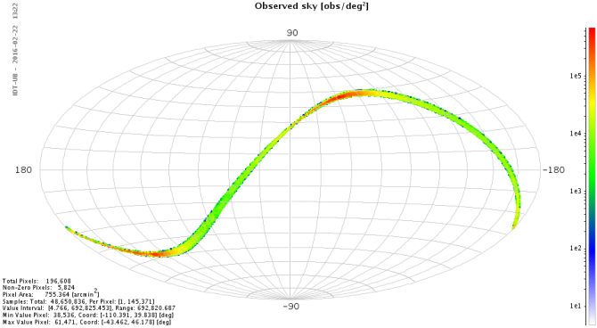
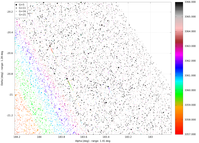
Figure 2.19: Example of sky region diagnostics in IDT, with a Mollweide projection of the density of transits processed during the last few hours (top panel, in transits per square degree, in equatorial coordinates), and a sky chart with the detections, times (in colour) and brightness (in the size of the dots) observed around a specific region (bottom panel). -
–
-
•
Photometric features (Figure 2.20):
-
–
Distribution of the number of transits per magnitude, in the , , , and bands.
-
–
‘Colour’ distribution, showing the transits per pseudo-colour, per effective wavelength, etc. Also colour-colour plots are determined, showing the effective wavelength distribution per colour.
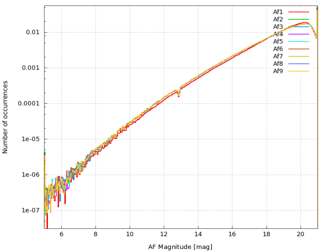
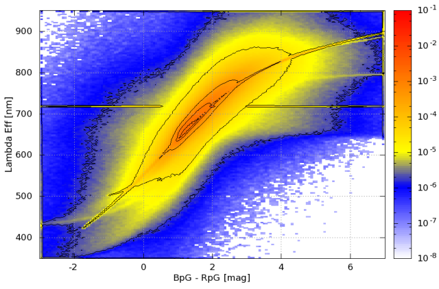
Figure 2.20: Example of transits density per -mag (top panel), which illustrates the exponential increase in star density with magnitude. The 2D histogram in the bottom panel illustrates the correlation between some of the preliminary colour features found by IDT, namely, the effective wavelength (which in turn correlates with the star temperature) and a colour index (based on the magnitude difference between the and bands). -
–
-
•
Attitude diagnostics (Figure 2.21, Figure 2.22, and Figure 2.23):
-
–
Distribution of match distances between the detections used by OGA1 and their associated sources.
-
–
Average number of detections per second used in the OGA1 attitude reconstruction.
-
–
Time series with the difference, in field angles (along and across scan), between the reconstructed attitude (OGA1) and the raw or IOGA attitudes. Also time series with the attitude rates (along and across scan) are determined.
-
–
Motions estimated for the transits processed, determined from the AF observation times and the attitude rates.
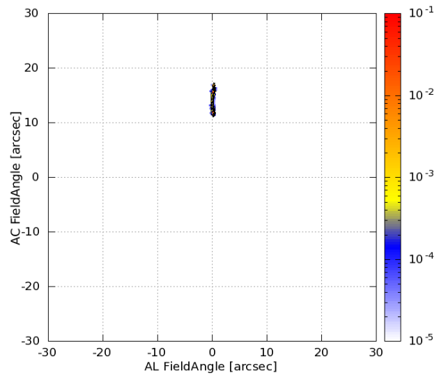
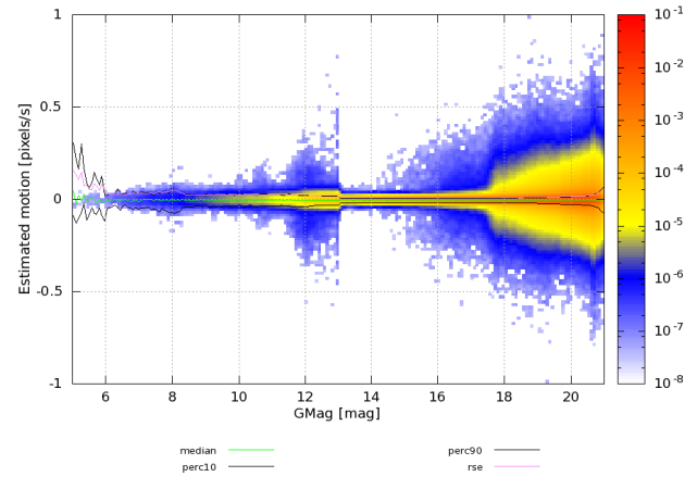
Figure 2.21: The top panel shows a distribution of match distances (in field angles) between the detections used in OGA1 and their associated stars. The bottom panel shows some results of the motions estimated for transits processed by IDT (in pixels per second, where 1 pixel per second means 60 mas s) as a function of the -mag estimated on-board. 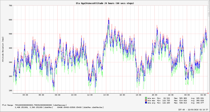
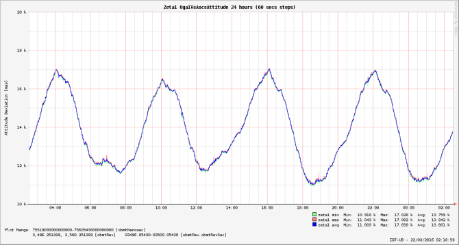
Figure 2.22: Difference between the first on-ground attitude refinement (OGA1) and the raw attitude determined on-board, which can be interpreted as the correction to be applied to such a raw attitude. It is shown for the along-scan field angle (top panel) and for one of the across-scan angles (bottom panel). The 6-hour periodicity is due to small variations in the alignment between the star tracker and the payload module. 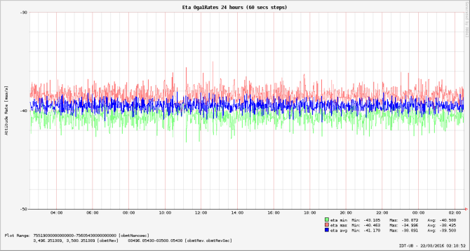
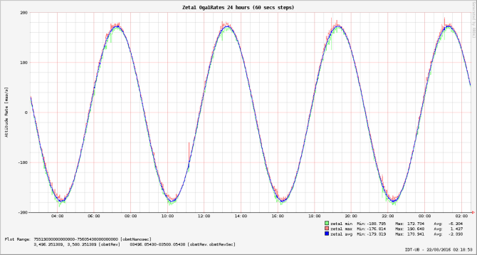
Figure 2.23: Along-scan (top panel) and across-scan (bottom panel) rates determined from OGA1. Along-scan rates help identifying clanks and micro-meteoroid impacts on the spacecraft. Across-scan variations are caused by precession of the spin axis. -
–
-
•
Bias diagnostics (Figure 2.24):
-
–
Histograms with the distribution of bias and readout noise values per CCD.
Figure 2.24: IDT snapshot showing the readout noise levels per CCD (larger image available). -
–
-
•
Background diagnostics (Figure 2.25):
-
–
Histograms with the astrophysical background level (in electrons per pixel per second) determined per CCD.
Figure 2.25: IDT snapshot showing the astrophysical background levels determined per CCD. Some CCDs show higher levels as a result of stray light (larger image available). -
–
-
•
Image parameters diagnostics (Figure 2.26):
-
–
Outcome of the Image Parameter Determination (IPD), indicating the fraction of windows with problems in the fitting.
-
–
Distribution of the ‘centroiding’ position within the SM or AF window, revealing possible problems in the on-board centring of the windows or in the PSF/LSF calibration.
-
–
Goodness-of-fit distribution, based on a estimation.
-
–
Distribution of formal errors in the fitting, as provided by the algorithm itself.
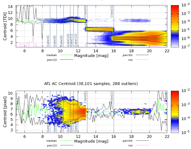
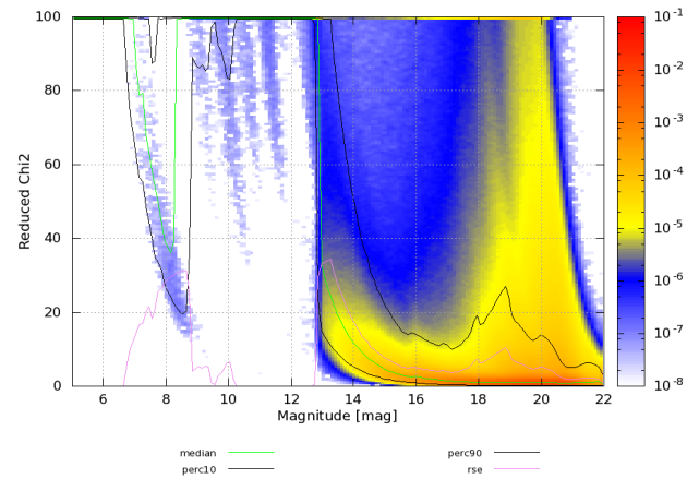
Figure 2.26: Top and middle panels: example of the centroid distribution determined for a given CCD (AF1 in this case), along (top) and across scan (middle), within the acquisition window, as a function of the on-board magnitude estimation. It illustrates the different sampling scheme depending on brightness. Bottom panel: goodness-of-fit in the astrometric image parameter determination, which shows reasonable fits for 1D windows (faint detections) and worse fits for bright detections due to the simplistic 1D 1D (AC AL) PSF model used in IDT. -
–
-
•
Crossmatching diagnostics (Figure 2.27):
-
–
Number of matched and unmatched transits (that is, detections for which no source has been found in the catalogue at a distance closer than 1.5 arcsec), number of detections identified as ‘spurious’, and number of new source entries created.
-
–
Distribution of match distances in the along- and across-scan directions.
-
–
Ambiguity in the crossmatch solution, indicating the fraction of transits for which more than one candidate source was found.
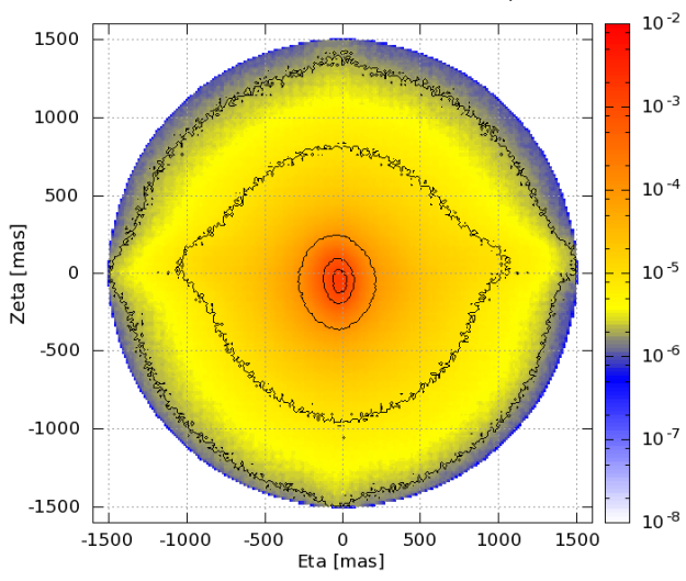
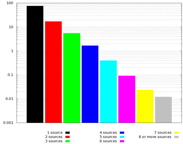
Figure 2.27: Top panel: distribution (in field angles) of the match distance in the daily crossmatch, revealing some features due to on-board spurious detections. Bottom panel: ambiguity in the crossmatch solution from IDT. -
–
First-Look diagnostics (FL)
Scientists processing data collected by astrometric space missions like Gaia have to simultaneously determine a large number of parameters concerning astrometry (and other stellar properties), the satellite’s attitude, as well as the geometric, photometric, and spectroscopic calibration of the instruments. To reach the inherent level of precision for Gaia, many months of observational data have to be incorporated in a global, coherent, and interleaved data reduction. Neither the instrument nor the data health can be verified at the desired level of precision by standard procedures applied to typical space missions. Obviously, it is undesirable not to know the current measurement precision and instrument stability until the next iteration in the global data processing is performed. Unperceived, subtle effects could arise and accumulate over time, irrevocably damaging the raw observations and resulting in a quality reduction or even loss of many months of science data. For this reason, a ‘First Look’ system was installed to judge the level of precision of the (astrometric, photometric, and spectroscopic) stellar, attitude, and instrument calibration parameters on a daily basis and to achieve its targeted performance level by means of sophisticated monitoring and evaluation of the observational data. These daily checks include analyses of:
-
•
astrometric science data with the help of the so-called One-Day Astrometric Solution (ODAS), which allows to derive an accurate on-ground attitude, improved source parameters, daily geometric instrument parameters as well as astrometric residuals required to assess the quality of the daily astrometric solution,
-
•
photometric and spectroscopic science data in order to assess the CCD health and the sanity of the LSF/PSF and spectroscopic calibrations,
-
•
the basic-angle monitor (BAM) data which aims at independently checking the behaviour of the Gaia basic angle,
-
•
auxiliary data such as on-board data needed to allow for a proper science data reduction on ground and on-board processing counters which allow to check the sanity of the on-board processing, and
-
•
the satellite housekeeping data.
The First Look aims at a quick discovery of, sometimes delicate, changes in the spacecraft and payload performance, but also aims at identifying oddities and proposing potential improvements in the initial steps of the on-ground data reduction. Its main goal is to influence the mission operations if and when need arises. The regular products and activities of the First-Look system and team include:
-
•
The One-Day Astrometric Solution (ODAS), which allows to derive a high-precision on-ground attitude, high-precision star positions, and a detailed daily geometric calibration of the astrometric instrument. The ODAS is by far the most complex part of the First-Look system.
-
•
Astrometric residuals of the individual ODAS measurements, required to assess the quality of the measurements and of the daily astrometric solution.
-
•
An automatically generated daily report of typically more than 3000 pages, containing thousands of histograms, time evolution plots, number statistics, calibration parameters, etc.
-
•
A daily manual assessment of this report. This is made possible in about 1–2 hours by an intelligent hierarchical structure, extended internal cross-referencing, and automatic signalling of apparently deviant aspects.
-
•
Condensed, periodic reports on all findings of potential problems and oddities. These are compiled manually by the so-called First Look Scientists team and the wider Payload Experts Group (Section 1.2.2). If needed, these groups also propose actions to improve the performance of Gaia and of the data processing on ground. Such actions may include telescope refocussing, change of on-board calibrations and configuration tables, decontamination campaigns, improvements of the IDT configuration parameters, definition of break points in the calibrations, and many others.
-
•
Manual qualification of all First-Look data products used in downstream data processing (attitude, source parameters, and geometric instrument calibration parameters).
In this way, First Look ensures that Gaia achieves the targeted data quality, and also supports the cyclic processing systems by providing calibration data. In particular the daily attitude and star positions are used for the wavelength calibration of the photometric and spectroscopic instruments of Gaia. In addition, the manual qualification of First-Look products helps both IDT and the cyclic processing teams to identify and discriminate healthy and (partly) corrupt data ranges and calibrations. In this way, bad data ranges can either be omitted or subject to special treatment (possibly including a complete reprocessing) at an early stage.
Astrometric Instrument Model (AIM) diagnostics
The main objective of the AIM system is the independent verification of selected AF monitoring and diagnostics, of the image parameters determination, instrument modelling, and calibration. AIM can be considered as a scaled-down counterpart of IDT (see Section 2.4.2) and FL (see Section 2.5.2) restricted to some astrometric elements of the daily processing, namely those that are particularly relevant for the astrometric error budget. This separate processing chain runs in Gaia DR2 with the following six modules: (Astrometric) Raw Data Processing, Selection, Monitoring, Daily Calibration, CalDiagnostic, and Report; in addition, several CalDiagnostic tasks run off-line. Each AIM processing step can be divided into three main parts: input, processing, and output.
Raw Data Processing
The main goal of the Raw Data Processing (RDP) is the determination of image parameter like AL and AC centroid, formal errors, flux, and background. A high-density-region filter runs before starting RDP when the satellite scans along the Galactic plane (Section 1.1.5) to process only the useful observations for the other AIM processing steps. The goal is to maintain the AIM capability to give a quick feedback on the astrometric instrument health and data reduction issues, if any.
The RDP inputs are the raw data (see Section 2.2.2) and selected outputs of the IDT system, namely:
-
•
AstroObservations with window class 0 and 1, i.e., stars brighter than mag;
-
•
PhotoElementaries.
The RDP outputs are the image parameters, i.e., centroid, formal errors, flux, and local background, all stored within AimElementaries. This allows routine comparisons with — and thus external verification of — IDT centroid values and corresponding formal errors. There are also specific inputs for the Monitoring processing.
Selection
The selection module selects those observations suitable for performing daily calibration. Indeed, for image profile reconstruction, only well-behaved observations must be selected, spread over the whole AIM -magnitude range. This means observations far from a charge injection event (more than 30 TDI lines) and with good image parameter fit results.
The inputs of the selection module are:
-
•
AstroObservations;
-
•
PhotoElementaries;
-
•
AstroElementaries;
-
•
AimElementaries.
The outputs are SelectionItems.
Monitoring
Monitoring is a collection of software modules, each dedicated to performing a particular task on selected data sets with the goal to extract information about instrument health, instrument calibration parameters, and image quality during in-flight operations over a few transits or much longer time scales.
Monitoring inputs are:
-
•
AimElementaries;
-
•
MonitorDiagnOutputs;
-
•
AstroObservations and AstroElementaries.
Monitoring outputs are plots and statistics, among which:
-
•
AIM centroid;
-
•
Formal errors AC and AL versus magnitude for each CCD;
-
•
AIM centroid residual variation AL and AC versus magnitude for each CCD;
-
•
AIM centroid residual variation AL and AC versus time for each CCD;
-
•
AIM image moment distributions over each row for each spectral bin;
-
•
Detection numbers for each magnitude and wavelength bin;
-
•
AIM AC and AL centroid mean variation over the row for each wavelength bin;
-
•
AIM AC and AL centroid mean variation over time and wavelength versus strips;
-
•
Comparison among AIM and IDT centroids;
-
•
Formal errors.
Daily Calibration
Two of the key Gaia calibrations are the reconstruction of the Line and Point Spread Functions (LSF/PSF). For that reason, AIM implements its own, independent Gaia signal profile reconstruction on a daily basis. The PSF/LSF image profile model is based, in a one-dimensional case, on a set of monochromatic basis functions, where the zero-order base is the sinc function squared, which depends on an non-dimensional argument , related to the focal plane coordinate , the wavelength , and the along-scan aperture width of the primary mirror. This corresponds to the signal generated by a rectangular, infinite slit of size , in the ideal (aberration-free) case of a telescope with effective focal length :
| (2.36) |
The contribution of finite pixel size, Modulation Transfer Function (MTF), and CCD operation in time-delay integration (TDI) mode are also included. The higher-order functions are generated by suitable combinations of the parent function and its derivatives according to a construction rule ensuring orthonormality by integration over the domain. The polychromatic functions are built according to linear superposition of the monochromatic counterparts, weighted by the normalized detected source spectrum which includes the response of the system.
The spatially variable LSF/PSF is reconstructed as the sum of spatially invariant functions, with coefficients varying over the field to describe the instrument response variation for sources of a given spectral distribution. The function basis is tuned to the actual characteristics of the signal by using a weighting function built from suitable data samples (Gai et al. 2013). The profile reconstruction is obtained using at most 11 terms for 1D profiles and between 30 and 65 terms for full 2D windows. Only the 1D profile reconstruction ran during the time interval covered by Gaia DR2. The upper limit of the astrometric error introduced by the fitting process for the 1D reconstruction is less than pixels, while the photometric error in is less than mag.
The ’astrometric error’ is the systematic error in the image position determination and the ’photometric error’ is the flux loss or flux gain using the selected model for the image flux determination. They are injected as a residual by the fit process which aims at reconstructing the image profile by building the template for the selected data set.
The modelling is based on 11 ad-hoc basis functions derived from a (simplified) physical representation of the opto-electronic system. The basis functions depend on just two tuning parameters. Checks are hence needed to ensure that the model is robust and that the correct solution for each template unit is chosen as the one which introduces a negligible ’astrometric’ bias, i.e., a negligible error on the position determination. This bias may be taken as the residual mismatch between the data set and its fit (but this is not the astrometric or photometric error on the elementary exposure or on Gaia’s final accuracy). With a goal of reaching a final astrometric accuracy of 10 as and milli-magnitude photometry, systematic errors need to be an order of magnitude smaller. A good solution for each bin (i.e., the LSF template for that bin) is the one that introduces an ’astrometric’ error and a ’photometric’ error below a given threshold. All templates combined realize the LSF library.
An AIM LSF/PSF library contains a calibration for each combination of telescope, CCD, source colour (wavelength for Gaia DR2), and AC motion. The LSF/PSF calibration will improve during the mission, with each processing calibration cycle.
The Daily Calibration inputs are:
-
•
AimElementaries;
-
•
SelectionItems;
-
•
MonitDiagnosticOutputs;
-
•
LsfsForLasAL;
-
•
LsfsForLasAC;
-
•
AstroElementaries;
-
•
CalibrationFeatures.
The Daily Calibration outputs are the results of the fitting procedure:
-
•
CalModulesResultsAL and CalModulesResultsAC;
-
•
CcdCalFlag;
-
•
The LSF library InstrImageFitLibrariesAL and InstrImageFitLibrariesAC.
CalDiagnostic
The CalDiagnostic inputs are the outputs from the Daily Calibration:
-
•
CalModulesResultsAL;
-
•
CalModulesResultsAC.
The CalDiagnostic outputs are plots and statistics, among which:
-
•
Focal plane average image quality variation for each AIM run which includes variation with colours over the row;
-
•
Average colour variation over the row;
-
•
Variation with colours over the strip;
-
•
Average colour variation over the strip;
-
•
Calibrated PSF template coefficient variation over the row depending on colours, which includes template moments variation over the row depending on colours;
-
•
Template moments variation over the row averaged over colours.
There are also a few tasks which perform trend analyses of the PSF/LSF image moments variations over weekly, monthly, and longer time intervals.
The AIM system uses an internal, automatic validation/qualification of the processing steps results, but manual inspection is needed for some particular outputs such as, for example, those coming from the comparison tasks with the main pipeline outputs.
Each day, a report is automatically produced collecting plots and statistics about raw data processing, calibration, and instrument health monitoring and diagnostics. These daily reports contain thousands of pages and are for internal use only. When needed, a condensed report about the findings of potential problems is sent to the Payload Experts group (Section 1.2.2). In this way, the AIM team supports the cyclic processing systems. No data produced by the Astrometric Instrument Model software entered Gaia DR2.
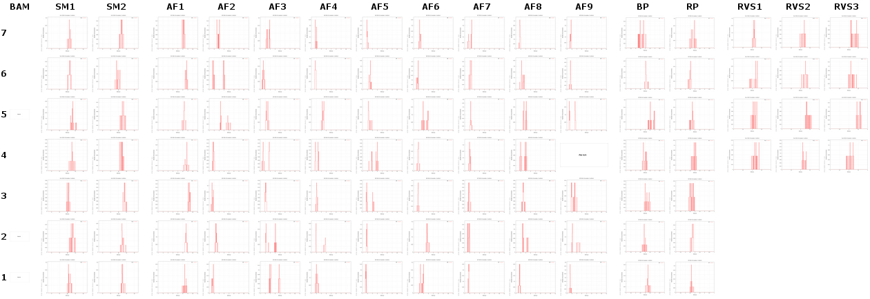
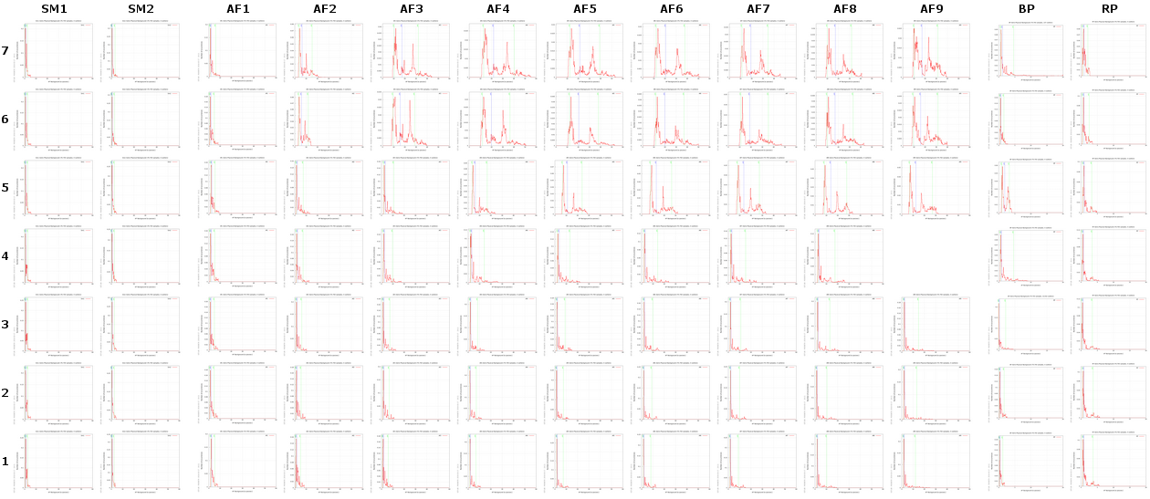
Basic Angle Monitoring (BAM) diagnostics
The BAM instrument (Section 1.1.3) is an interferometer monitoring the variation of the basic angle between the two telescopes (Section 1.1.3) by looking at the phase changes of the fringes (see also Section 2.4.4 and Gaia Collaboration et al. 2016). The AVU/BAM system monitors, on a daily basis, the BAM instrument and the basic angle variation (BAV), independently from IDT (see Section 2.4.2) and FL (see Section 2.5.2). AVU/BAM provides periodic reports, for evaluation by the Payload Experts group (Section 1.2.2) and for information of relevant groups in DPAC (AGIS, GSR, and FL), trend analyses on short and long time scales, calibrated BAV measurements (since December 2014), as well as a model of the temporal variations of the basic angle.
AVU/BAM is a fundamental component of the technical and scientific verification of the overall Gaia astrometric data processing and has been developed within the context of the Astrometric Verification Unit (AVU). Deployment and execution of the operational system is done at the Torino Data Processing Centre, DPCT (Section 1.3.4).
The input data to AVU/BAM (coming from DPCE; Section 1.3.4) correspond to a central region of the fringe envelope for each line of sight. For Gaia DR2, the central region corresponds to a matrix of samples (AL AC). Each of the 80 AC samples is binned on-board (using 4 physical pixels per sample). BAM CCDs are red-variant CCDs (as used in RP) and have a pixel size of m (AL AC).
AVU/BAM, besides producing the fundamental BAM measurements (e.g., time series of the phase variation), processes the elementary signal and provides an interpretation in terms of a physical model to allow early detection of unexpected behaviour of the system (e.g., trends and other systematic effects). The AVU/BAM pipeline performs two different kinds of analysis: the first is based on daily runs while the second is focussed on overall statistics on a weekly/monthly basis.
The most important output of AVU/BAM is an estimate of the differential basic angle variation (BAV) with time. The pipeline provides this BAV estimate through three different algorithms (described in Riva et al. 2014). The first algorithm, named Raw Data Processing (RDP, similar to the IDT approach), provides the BAV as the difference of the variation of the two lines of sight. Each line-of-sight estimate is performed through a cross correlation of each BAM image with a template composed of the mean of the first 100 images of each run. The second algorithm, named Gaiometro, is the 1D direct cross correlation between the two lines of sight. The third algorithm, called Gaiometro 2D, is a 2D version of the direct measurement of the BAV. The first two algorithms use images binned across scan. The four independent results (three from AVU/BAM plus the one from IDT) agree well in general, providing similar shapes of the 6-hour basic-angle oscillations, although the derived amplitudes differ at the level of 5 percent. It is as yet unknown which of the four methods gives the most faithful representation of the actual variations in the basic angle of the astrometric instrument.
In addition to producing time series of the fringe phase variations, AVU/BAM also makes measurements of other basic quantities characteristic of the BAM instrument, like fringe period, fringe flux, and fringe contrast. The fringe flux is calculated as the raw pixel sum of each frame. The fringe period is given by:
| (2.37) |
with the telescope focal length, the wavelength, and the BAM baseline. The fringe contrast is related to the visibility of the fringes. The temporal variations of these quantities are monitored and analysed to support the BAV interpretation.
No data produced by the AVU/BAM software has entered Gaia DR2.