2.3.2 Early PSF/LSF model
Author(s): Michael Davidson, Lennart Lindegren
Two of the key Gaia calibrations are the Line Spread Functions (LSF) and Point Spread Functions (PSF). These are the profiles used to determine the image parameters for each window in a maximum-likelihood estimation (see Section 2.4.8), specifically the along-scan (AL) image location (observation time), source flux, plus across-scan location in the case of 2D windows. Of these, the observation time is of greatest importance in the astrometric solution, and this is reflected in the higher requirements on the AL locations when compared to the AC locations (Lindegren et al. 2012). Indeed, to increase the signal-to-noise, the majority of windows are binned in the across-scan direction and are observed as 1D profiles. A Line Spread Function is thus more useful than a 2D Point Spread Function in these cases. The PSF is often understood as the response of the optical system to a point impulse, however in practice for Gaia it is more useful to include also effects such as the finite pixel size, TDI smearing, and charge diffusion. This leads to the concept of the effective PSF, as introduced in Anderson and King (2000). Pixelisation and other effects are thereby included directly within the PSF profiles.
Calibration of the LSF/PSF is among the most challenging tasks in the overall Gaia data processing, due to the dependence on other calibrations, such as the background and CCD health, and due to uncertainties in crucially measured inputs like colour. This calibration will also become more difficult as radiation damage to the detectors increases through the mission, causing a non-linear distortion. Discussion of these CTI effects can be found in Fabricius et al. (2016) and in Section 1.3.3 and Section 1.3.3. Here, we focus on the LSF/PSF of the astrometric instrument, which in the pre-processing step is assumed to be linear, allowing a more straightforward modelling and application. The LSF/PSF varies over the relatively wide field of view of each telescope (17 07) and with the spectral energy distribution of the observed source. As previously discussed, the observation time of a source depends on the TDI gate used and, since the LSF/PSF profile can vary along even a single CCD, all gate configurations must be calibrated independently. This can be difficult for the shortest gates due to the relatively low number of observations available. An LSF/PSF library contains a calibration for each combination of telescope, CCD, and gate.
Several aspects must be considered when defining a model to represent the LSF/PSF. Firstly, the LSF profiles must be continuous in value and derivative, and they must be non-negative. By definition, the full integral in the AL direction is 1, thus neglecting the flux lost above and below the binned AC window. This AC flux loss is calibrated as part of the photometric system. The LSF response is normalised as:
| (2.1) |
where is the LSF origin. The origin should be chosen to be achromatic (the centroid of a symmetrical LSF is aligned with the origin but this is not true in general), and since image locations are measured relative to it, it should be tied to a physically well-defined celestial direction. However, it is not possible to separate geometric calibration from chromaticity effects within the daily pipeline; this requires the global astrometric solution from the cyclic processing. The origin is therefore fixed as and, consequently, there will be a colour-dependent bias in this internal LSF calibration. The LSF profile is used to model the expected, de-biased photo-electron flux of a single stellar source, including noise, by:
| (2.2) |
where , , and are the background level, the flux of the source, and the along-scan image location. The index is the along-scan location of the CCD sample under consideration. The actual photo-electron counts will include a random noise component, in addition.
For the practical application, the LSF can be modelled as a linear combination of basis components:
| (2.3) |
where basis functions are used. The value of each basis function at coordinate is scaled by a weight appropriate for the given observation. A set of basis functions can be derived through Principal Component Analysis (PCA) of a collection of LSF profiles chosen to represent the actual spread of observations, i.e., covering all devices and a wide range of source colours and across-scan smearing rates. An advantage of PCA is that the basis functions are ranked by significance, allowing selection of the minimum number of components required to reach a particular level of residuals. These basis functions can, in turn, be chosen in a variety of ways; we have used an S-spline model (see Section 2.3.2) with a smooth transition to Lorentzian profiles at the LSF wings. Further optimisation can be achieved to assure the correct normalisation by transforming these bases, although this is beyond the scope of the current document. A set of 51 basis functions were determined from pre-flight simulation data, each represented using 75 coefficients. The 20 most significant functions have been found to adequately represent real LSFs, although further improvements are possible.
With a given set of basis functions , the task of LSF calibration becomes the determination of the basis weights . These weights depend on the observation parameters including AC position within the CCD, effective wavelength, AC smearing, and others. In general, the observation parameters can be written as a vector and the weights thus as . To allow smooth interpolation, each basis weight can be represented as a spline surface where each dimension corresponds to an observation parameter. In the actually implemented calibration system, each dimension can be configured separately with sufficient flexibility to accommodate the actual structure in the weight surface, i.e., via choice of the spline order and knots. In practice, the number of observation parameters has been restricted to two: AC position and effective wavelength (i.e., source colour) for AL LSF, and AC smearing and effective wavelength for the AC LSF. The coefficients of the weight surface are formed from the outer product of two splines with and coefficients respectively. There are therefore weight parameters per basis function which must be fitted.
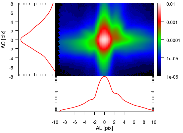
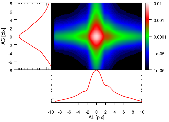
The rectangular telescope apertures in Gaia led to a simple model to approximate the PSF in the daily pipeline. The PSF is formed by the cross product of the AL and AC LSFs. This model has a relatively small number of parameters to fit at the price of being unable to represent all the structure in the PSF. We have confirmed that the AC AL approximation does not introduce significant bias into the measured observation times for 2D windows. Experiments to compare the fitted observation times using the AC AL versus a full 2D PSF indicate a systematic bias of pixels. An example of the PSF and its reconstruction via the AC AL model is presented in Figure 2.1 and Figure 2.2.
LSF calibrations are obtained by selecting so-called calibrator observations. These are chosen to be healthy (e.g., nominal gate, regular window shape) and not affected by charge injections or rapid charge release. Image parameter and colour estimation for the observation must be successful; good bias and background information must be available. With these data, Equation 2.2 can be used to provide an LSF measure per unmasked sample. In the case of 2D windows, the observation is binned in the AL or AC direction as appropriate to give LSF calibrations. The quantity of data available varies with calibration unit. Note that a ‘calibration unit’ in the Gaia pipeline is a given combination of window class (e.g., 1D or 2D), gate, CCD, telescope, possibly time interval (days, weeks, months), and possibly other parameters, e.g., AC coordinate interval on a CCD. For the most common configurations (faint un-gated windows), there are many more eligible observations than can be handled, thus a thinned-out selection of calibrators is used.
A least-squares method is used with the LSF calibrations to fit the basis weight coefficients. The Householder least-squares technique is useful here as it allows calibrators to be processed in separate time batches and for their solutions to be merged. The merger can also be weighted to enable a running solution to track changes in the LSFs over time (see van Leeuwen 2007a). Various automated and manual validations are performed on an updated LSF library before approval is given for it to be used by the daily pipeline for subsequent image parameter determination. There are checks on each solution to ensure that the goodness-of-fit is within the expected range, that the number of degrees-of-freedom is sufficiently positive, and that the reconstructed LSFs are well-behaved over the necessary range of . Individual solutions may be rejected and the corresponding existing ‘best-available’ solution be carried forward. In this way, an operational LSF library always has a full complement of solutions for all devices and nominal configurations.
The LSF solutions are updated daily within the real-time system, although they are not approved for use at that frequency. Indeed, a single library generated during commissioning has been used throughout the period covered by this second Gaia data release, in order to provide stability in the system during the early mission. This library has a limited set of dependencies including field-of-view and CCD, but it does not include important parameters such as colour, AC smearing, or AC position within a CCD. As such, it is essentially a library of mean LSFs and AC AL PSFs. This will change for future Gaia data releases.
S-spline representation of the LSF
This section motivates and defines the special kind of spline functions, here called S-splines, used to represent the cores of the Line Spread Functions (LSFs) via the basis functions (see Section 2.3.2). In some earlier, mostly DPAC-internal documentation, the S-splines have erroneously been called ’bi-quartic’ splines; however, that term should be reserved for two-dimensional quartic splines, and may be particularly confusing in the context of PSF modelling. In Prod’homme et al. (2012), the S-spline is referred to as a ’special quartic spline’.
A physically realistic model of the LSF should satisfy a number of constraints, including non-negativity () and that it is everywhere continuous in value and derivative. Since diffraction is involved, one can also expect that spatial frequencies above are negligible, where m is the along-scan size of the entrance pupil and nm the short-wavelength cut-off. The effective LSF, which includes pixelisation (Section 2.3.2), should in addition satisfy the shift-sum invariance condition:
| (2.4) |
where is the pixel size. This condition immediately follows from the conservation of energy: the intensity of the image corresponds to the total number of photons, independent of the precise location of the image with respect to the pixel boundaries. Numerical experiments indicate that the fitted LSF model should be shift-sum invariant in order to avoid estimation biases as function of sub-pixel position.
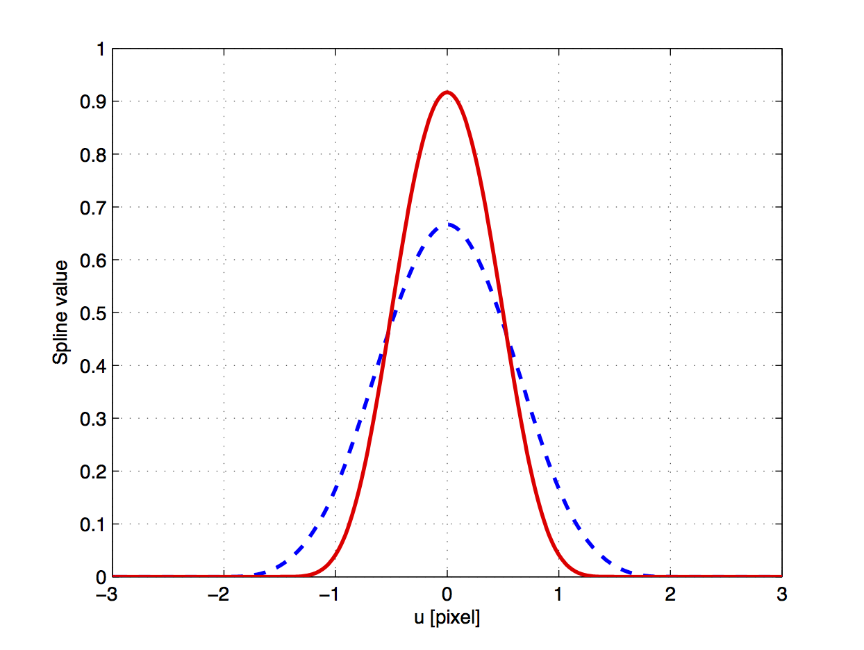
A cubic spline is a piecewise polynomial function that is continuous in value and first two derivatives. It is naturally smooth, and therefore to some degree band-limited, and the non-negativity constraint can be enforced by the fitting procedure. A cubic spline defined on a regular knot sequence with knot separation is, moreover, strictly shift-sum invariant, and would thus appear to be ideal for the LSF modelling. Unfortunately, it turns out that a cubic spline with knot separation is not always flexible enough to represent the core of the LSF for Gaia. The basic reason for this is that the optical images in Gaia are undersampled by the CCDs: , while the sampling theorem requires . Increasing the order of the spline does not help: it makes the spline smoother, but not more flexible.
To obtain greater flexibility, it is necessary to decrease the knot interval, but then the shift-invariance condition is in general not satisfied. However, among the splines that use a fixed knot interval (for integer ), there exists a subset of splines that do respect the shift-sum condition. These are the S-splines. The simplest way to construct an S-spline is to take an ordinary spline of order , defined on a regular knot sequence with knot interval , and convolve it with a rectangular (boxcar) function of width . It is readily seen that the result is a spline of order , with the same knot interval as the original spline, but respecting the shift–sum invariance. Since the original spline can be expressed as a linear combination of B-splines (splines with minimal support), the S-spline can be expressed as a linear combination of B-splines convolved with the rectangular function.
The S-splines used to represent the cores of the basis functions , and hence of , were obtained with and . They are thus quartic splines defined of a regular knot sequence with knot separation , and can be written as a linear combination of the functions , where
| (2.5) |
for . Alternatively, can be obtained by adding two adjacent quartic B-splines. Figure 2.3 shows this function together with the cubic B-spline for knot interval . Although both functions satisfy Equation 2.4, the S-spline can clearly represent peaks of the LSF that are narrower than is possible with the B-spline. Other choices than and are possible but have not been tested.
While the decomposition of a given spline in terms of B-splines is always unique, the decomposition in terms of is not necessarily unique. This is not a problem as long as the coefficients of are not directly used to parametrise the LSF, but are only used to represent pre-defined basis functions such as . When fitting an S-spline to , the possible non-uniqueness of the coefficients can be handled by using the pseudo-inverse.